Option Explicit
Sub Macro1()
'
' Macro1 Macro
'
' Keyboard Shortcut: Ctrl+q
'
Sheets("Sheet1").Select
Range("A1:L26").Select
Selection.Copy
Sheets("Sheet2").Select
Range("A1").Select
Selection.PasteSpecial Paste:=xlPasteAll, Operation:=xlNone, SkipBlanks:= _
False, Transpose:=True
End Sub
Sub Macro2()
'
' Macro2 Macro
'
'
Sheets("Sheet3").Select
Application.CutCopyMode = False
Selection.Copy
Sheets("Sheet2").Select
Selection.SpecialCells(xlCellTypeBlanks).Select
ActiveSheet.Paste
Application.CutCopyMode = False
End Sub
Sub Macro3()
'
' Macro3 Macro
'
'
Sheets("Sheet2").Select
Range("B1").Select
Range(Selection, Selection.End(xlDown)).Select
Selection.Cut
Range("A1").Select
Range(Selection, Selection.End(xlDown)).Select
Selection.End(xlDown).Select
ActiveCell.Offset(1, 0).Range("A1").Select
ActiveSheet.Paste
Range("C1").Select
Range(Selection, Selection.End(xlDown)).Select
Selection.Cut
Range("A1").Select
Range(Selection, Selection.End(xlDown)).Select
Selection.End(xlDown).Select
ActiveCell.Offset(1, 0).Range("A1").Select
ActiveSheet.Paste
Range("D1").Select
Range(Selection, Selection.End(xlDown)).Select
Selection.Cut
Range("A1").Select
Range(Selection, Selection.End(xlDown)).Select
Selection.End(xlDown).Select
ActiveCell.Offset(1, 0).Range("A1").Select
ActiveSheet.Paste
Range("E1").Select
Range(Selection, Selection.End(xlDown)).Select
Selection.Cut
Range("A1").Select
Range(Selection, Selection.End(xlDown)).Select
Selection.End(xlDown).Select
ActiveCell.Offset(1, 0).Range("A1").Select
ActiveSheet.Paste
Range("F1").Select
Range(Selection, Selection.End(xlDown)).Select
Selection.Cut
Range("A1").Select
Range(Selection, Selection.End(xlDown)).Select
Selection.End(xlDown).Select
ActiveCell.Offset(1, 0).Range("A1").Select
ActiveSheet.Paste
Range("G1").Select
Range(Selection, Selection.End(xlDown)).Select
Selection.Cut
Range("A1").Select
Range(Selection, Selection.End(xlDown)).Select
Selection.End(xlDown).Select
ActiveCell.Offset(1, 0).Range("A1").Select
ActiveSheet.Paste
Range("H1").Select
Range(Selection, Selection.End(xlDown)).Select
Selection.Cut
Range("A1").Select
Range(Selection, Selection.End(xlDown)).Select
Selection.End(xlDown).Select
ActiveCell.Offset(1, 0).Range("A1").Select
ActiveSheet.Paste
Range("I1").Select
Range(Selection, Selection.End(xlDown)).Select
Selection.Cut
Range("A1").Select
Range(Selection, Selection.End(xlDown)).Select
Selection.End(xlDown).Select
ActiveCell.Offset(1, 0).Range("A1").Select
ActiveSheet.Paste
Range("J1").Select
Range(Selection, Selection.End(xlDown)).Select
Selection.Cut
Range("A1").Select
Range(Selection, Selection.End(xlDown)).Select
Selection.End(xlDown).Select
ActiveCell.Offset(1, 0).Range("A1").Select
ActiveSheet.Paste
Range("K1").Select
Range(Selection, Selection.End(xlDown)).Select
Selection.Cut
Range("A1").Select
Range(Selection, Selection.End(xlDown)).Select
Selection.End(xlDown).Select
ActiveCell.Offset(1, 0).Range("A1").Select
ActiveSheet.Paste
Range("L1").Select
Range(Selection, Selection.End(xlDown)).Select
Selection.Cut
Range("A1").Select
Range(Selection, Selection.End(xlDown)).Select
Selection.End(xlDown).Select
ActiveCell.Offset(1, 0).Range("A1").Select
ActiveSheet.Paste
Range("M1").Select
Range(Selection, Selection.End(xlDown)).Select
Selection.Cut
Range("A1").Select
Range(Selection, Selection.End(xlDown)).Select
Selection.End(xlDown).Select
ActiveCell.Offset(1, 0).Range("A1").Select
ActiveSheet.Paste
Range("N1").Select
Range(Selection, Selection.End(xlDown)).Select
Selection.Cut
Range("A1").Select
Range(Selection, Selection.End(xlDown)).Select
Selection.End(xlDown).Select
ActiveCell.Offset(1, 0).Range("A1").Select
ActiveSheet.Paste
Range("O1").Select
Range(Selection, Selection.End(xlDown)).Select
Selection.Cut
Range("A1").Select
Range(Selection, Selection.End(xlDown)).Select
Selection.End(xlDown).Select
ActiveCell.Offset(1, 0).Range("A1").Select
ActiveSheet.Paste
Range("P1").Select
Range(Selection, Selection.End(xlDown)).Select
Selection.Cut
Range("A1").Select
Range(Selection, Selection.End(xlDown)).Select
Selection.End(xlDown).Select
ActiveCell.Offset(1, 0).Range("A1").Select
ActiveSheet.Paste
Range("Q1").Select
Range(Selection, Selection.End(xlDown)).Select
Selection.Cut
Range("A1").Select
Range(Selection, Selection.End(xlDown)).Select
Selection.End(xlDown).Select
ActiveCell.Offset(1, 0).Range("A1").Select
ActiveSheet.Paste
Range("R1").Select
Range(Selection, Selection.End(xlDown)).Select
Selection.Cut
Range("A1").Select
Range(Selection, Selection.End(xlDown)).Select
Selection.End(xlDown).Select
ActiveCell.Offset(1, 0).Range("A1").Select
ActiveSheet.Paste
Range("S1").Select
Range(Selection, Selection.End(xlDown)).Select
Selection.Cut
Range("A1").Select
Range(Selection, Selection.End(xlDown)).Select
Selection.End(xlDown).Select
ActiveCell.Offset(1, 0).Range("A1").Select
ActiveSheet.Paste
Range("T1").Select
Range(Selection, Selection.End(xlDown)).Select
Selection.Cut
Range("A1").Select
Range(Selection, Selection.End(xlDown)).Select
Selection.End(xlDown).Select
ActiveCell.Offset(1, 0).Range("A1").Select
ActiveSheet.Paste
Range("U1").Select
Range(Selection, Selection.End(xlDown)).Select
Selection.Cut
Range("A1").Select
Range(Selection, Selection.End(xlDown)).Select
Selection.End(xlDown).Select
ActiveCell.Offset(1, 0).Range("A1").Select
ActiveSheet.Paste
Range("V1").Select
Range(Selection, Selection.End(xlDown)).Select
Selection.Cut
Range("A1").Select
Range(Selection, Selection.End(xlDown)).Select
Selection.End(xlDown).Select
ActiveCell.Offset(1, 0).Range("A1").Select
ActiveSheet.Paste
Range("W1").Select
Range(Selection, Selection.End(xlDown)).Select
Selection.Cut
Range("A1").Select
Range(Selection, Selection.End(xlDown)).Select
Selection.End(xlDown).Select
ActiveCell.Offset(1, 0).Range("A1").Select
ActiveSheet.Paste
Range("X1").Select
Range(Selection, Selection.End(xlDown)).Select
Selection.Cut
Range("A1").Select
Range(Selection, Selection.End(xlDown)).Select
Selection.End(xlDown).Select
ActiveCell.Offset(1, 0).Range("A1").Select
ActiveSheet.Paste
Range("Y1").Select
Range(Selection, Selection.End(xlDown)).Select
Selection.Cut
Range("A1").Select
Range(Selection, Selection.End(xlDown)).Select
Selection.End(xlDown).Select
ActiveCell.Offset(1, 0).Range("A1").Select
ActiveSheet.Paste
Range("Z1").Select
Range(Selection, Selection.End(xlDown)).Select
Selection.Cut
Range("A1").Select
Range(Selection, Selection.End(xlDown)).Select
Selection.End(xlDown).Select
ActiveCell.Offset(1, 0).Range("A1").Select
ActiveSheet.Paste
End Sub
Sub Macro4()
'
' Macro4 Macro
'
'
Sheets("Sheet2").Select
Range("A1").Select
Range(Selection, Selection.End(xlDown)).Select
Selection.Cut
Sheets("Sheet4").Select
Range("A1").Select
ActiveSheet.Paste
Columns("A:A").Select
Selection.Insert Shift:=xlToRight, CopyOrigin:=xlFormatFromLeftOrAbove
Sheets("Sheet1").Select
Rows("1:26").Select
Selection.Delete Shift:=xlUp
End Sub
Showing posts with label excel macros. Show all posts
Showing posts with label excel macros. Show all posts
Wednesday, January 26, 2011


Wednesday, February 17, 2010
http://www.excelforum.com/excel-worksheet-functions/366493-how-do-i-use-vlookup-for-multiple-occurrences-of-the-same-value.html
I am using the vlookup function to check a table which may or may not have
multiple rows for the same value of the column I am using to select. So far,
everything I have tried keeps giving me the first occurrence it finds. Do I
need to add additional parameters or should I be using something other than
vlookup?
If you have the functions in the freely downloadable file at
http:/home.pacbell.net/beban available to your workbook you can use the
VLookups function:
=VLookups(lookup_value,Lookup_table,column_reference) array entered into
enough vertical cells to accommodate the number of occurrences of
lookup_value. Or, to avoid array entering:
=Index(VLookups(lookup_value,Lookup_table,column_reference), Row(A1))
filled down as far as required.
********************************************************
Option Explicit
Public Function vlookupall$(strSearch As String, rngRange As Range, lngLookupCol As Long)
'Vlookupall searches in first column of rngRange for strSearch and returns corresponding
'values of column lngLookupCol if strSearch was found. All corr. values are collected and
'returned in one string (result of function).
Dim i As Long
If lngLookupCol > rngRange.Columns.Count Then
vlookupall = CVErr(xlErrValue)
Exit Function
End If
vlookupall = ""
For i = 1 To rngRange.Rows.Count
If rngRange(i, 1).Text = strSearch Then
vlookupall = vlookupall & rngRange(i, lngLookupCol).Text & "; "
End If
Next i
End Function
http://www.sulprobil.com/html/vlookupall.html
I am using the vlookup function to check a table which may or may not have
multiple rows for the same value of the column I am using to select. So far,
everything I have tried keeps giving me the first occurrence it finds. Do I
need to add additional parameters or should I be using something other than
vlookup?
If you have the functions in the freely downloadable file at
http:/home.pacbell.net/beban available to your workbook you can use the
VLookups function:
=VLookups(lookup_value,Lookup_table,column_reference) array entered into
enough vertical cells to accommodate the number of occurrences of
lookup_value. Or, to avoid array entering:
=Index(VLookups(lookup_value,Lookup_table,column_reference), Row(A1))
filled down as far as required.
********************************************************
Option Explicit
Public Function vlookupall$(strSearch As String, rngRange As Range, lngLookupCol As Long)
'Vlookupall searches in first column of rngRange for strSearch and returns corresponding
'values of column lngLookupCol if strSearch was found. All corr. values are collected and
'returned in one string (result of function).
Dim i As Long
If lngLookupCol > rngRange.Columns.Count Then
vlookupall = CVErr(xlErrValue)
Exit Function
End If
vlookupall = ""
For i = 1 To rngRange.Rows.Count
If rngRange(i, 1).Text = strSearch Then
vlookupall = vlookupall & rngRange(i, lngLookupCol).Text & "; "
End If
Next i
End Function
http://www.sulprobil.com/html/vlookupall.html
Monday, February 15, 2010
Monday, February 8, 2010
Saturday, January 30, 2010
Macro to delete alternative rows
Sub DeleteEvenRows()
Application.ScreenUpdating = False
Dim i As Long
For i = Cells.SpecialCells(xlLastCell).Row To 2 Step -1
If i Mod 2 = 0 Then Rows(i).Delete
Next i
Application.ScreenUpdating = True
End Sub
Application.ScreenUpdating = False
Dim i As Long
For i = Cells.SpecialCells(xlLastCell).Row To 2 Step -1
If i Mod 2 = 0 Then Rows(i).Delete
Next i
Application.ScreenUpdating = True
End Sub
Tuesday, January 19, 2010
Monday, January 4, 2010
Excel: IF-THEN-ELSE Statement (VBA only)
--------------------------------------------------------------------------------
In Excel, the IF-THEN-ELSE statement can only be used in VBA code.
The syntax for the IF-THEN-ELSE statement is:
If condition_1 Then
result_1
ElseIf condition_2 Then
result_2
...
ElseIf condition_n Then
result_n
Else
result_else
End If
condition_1 to condition_n are evaluated in the order listed. Once a condition is found to be true, the IF-THEN-ELSE statement will execute the corresponding code and not evaluate the conditions any further.
result_1 to result_n is the code that is executed once a condition is found to be true.
Note:
If no condition is met, then the Else portion of the IF-THEN-ELSE statement will be executed.
It is important to note that the ElseIf and Else portions are optional.
Applies To:
Excel 2007, Excel 2003, Excel XP, Excel 2000
VBA Code
The IF-THEN-ELSE statement can only be used in VBA code.
First, let's take a look at a simple example.
If LRegion ="N" Then
LRegionName = "North"
End If
Next, let's take a look at an example that uses ElseIf.
If LRegion ="N" Then
LRegionName = "North"
ElseIf LRegion = "S" Then
LRegionName = "South"
ElseIf LRegion = "E" Then
LRegionName = "East"
ElseIf LRegion = "W" Then
LRegionName = "West"
End If
Finally, let's take a look at an example that uses Else.
If LRegion ="N" Then
LRegionName = "North"
ElseIf LRegion = "S" Then
LRegionName = "South"
ElseIf LRegion = "E" Then
LRegionName = "East"
Else
LRegionName = "West"
End If
--------------------------------------------------------------------------------
In Excel, the IF-THEN-ELSE statement can only be used in VBA code.
The syntax for the IF-THEN-ELSE statement is:
If condition_1 Then
result_1
ElseIf condition_2 Then
result_2
...
ElseIf condition_n Then
result_n
Else
result_else
End If
condition_1 to condition_n are evaluated in the order listed. Once a condition is found to be true, the IF-THEN-ELSE statement will execute the corresponding code and not evaluate the conditions any further.
result_1 to result_n is the code that is executed once a condition is found to be true.
Note:
If no condition is met, then the Else portion of the IF-THEN-ELSE statement will be executed.
It is important to note that the ElseIf and Else portions are optional.
Applies To:
Excel 2007, Excel 2003, Excel XP, Excel 2000
VBA Code
The IF-THEN-ELSE statement can only be used in VBA code.
First, let's take a look at a simple example.
If LRegion ="N" Then
LRegionName = "North"
End If
Next, let's take a look at an example that uses ElseIf.
If LRegion ="N" Then
LRegionName = "North"
ElseIf LRegion = "S" Then
LRegionName = "South"
ElseIf LRegion = "E" Then
LRegionName = "East"
ElseIf LRegion = "W" Then
LRegionName = "West"
End If
Finally, let's take a look at an example that uses Else.
If LRegion ="N" Then
LRegionName = "North"
ElseIf LRegion = "S" Then
LRegionName = "South"
ElseIf LRegion = "E" Then
LRegionName = "East"
Else
LRegionName = "West"
End If
http://www.techonthenet.com/excel/index.php
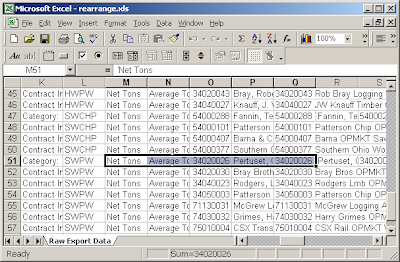
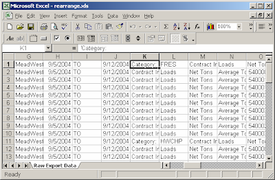
Excel: Rearrange data in an export of raw data in Excel 2003/XP/2000/97
--------------------------------------------------------------------------------
Question: In Excel 2003/XP/2000/97, I have a spreadsheet that contains an export of some raw data. However, the data needs to be rearranged as follows:
If cell M? displays "Contract Information" then copy and paste cells O-S into cell M of the same row
If cell K? displays "Location" then cut and paste cells K-AD into cell T of the same row. Then copy and paste the previous row's cells K-S down to K into this row
Copy down the category name in Column L replacing "Loads"
Answer: Let's take a look at an example.
Download Excel spreadsheet (as demonstrated below)
In this spreadsheet, we've created a macro called RearrangeData. You can run the macro by selecting Macro > Macros under the Tools menu. Then highlighting the macro called RearrangeData and clicking on the Run button.
Once the macro has run, the spreadsheet will look as follows:
You can press Alt-F11 to view the VBA code.
Macro Code:
The macro code looks like this:
Sub RearrangeData()
Dim LRow As Integer
Dim LCategory As String
LRow = 1
LCategory = ""
'Move through records until an empty cell is found in column A
While IsEmpty(Range("A" & CStr(LRow)).Value) = False
'If cell M? displays "Contract Information" then copy and paste
'cells O-S into cell M of the same row
If Range("M" & CStr(LRow)).Value = "Contract Information" Then
Range("O" & LRow & ":S" & LRow).Select
Selection.Copy
Range("M" & LRow).Select
ActiveSheet.Paste
End If
'If cell K? displays "Location" then cut and paste cells K-AD into
'cell T of the same row. Then copy and paste the previous row's
'cells K-S down to K into this row
If Range("K" & CStr(LRow)).Value = "Location" Then
'Cut and paste cells K-AD into cell T of the same row
Range("K" & LRow & ":AD" & LRow).Select
Selection.Cut
Range("T" & LRow).Select
ActiveSheet.Paste
'Copy and paste the previous row's cells K-S down to K
'into this row
Range("K" & LRow - 1 & ":S" & LRow - 1).Select
Selection.Copy
Range("K" & LRow).Select
ActiveSheet.Paste
End If
'Copy down the category name in Column L replacing "Loads"
If Range("L" & CStr(LRow)).Value = "Loads" Then
Range("L" & CStr(LRow)).Value = LCategory
'Next category name
Else
LCategory = Range("L" & CStr(LRow)).Value
End If
LRow = LRow + 1
Wend
End Sub


Excel: Rearrange data in an export of raw data in Excel 2003/XP/2000/97
--------------------------------------------------------------------------------
Question: In Excel 2003/XP/2000/97, I have a spreadsheet that contains an export of some raw data. However, the data needs to be rearranged as follows:
If cell M? displays "Contract Information" then copy and paste cells O-S into cell M of the same row
If cell K? displays "Location" then cut and paste cells K-AD into cell T of the same row. Then copy and paste the previous row's cells K-S down to K into this row
Copy down the category name in Column L replacing "Loads"
Answer: Let's take a look at an example.
Download Excel spreadsheet (as demonstrated below)
In this spreadsheet, we've created a macro called RearrangeData. You can run the macro by selecting Macro > Macros under the Tools menu. Then highlighting the macro called RearrangeData and clicking on the Run button.
Once the macro has run, the spreadsheet will look as follows:
You can press Alt-F11 to view the VBA code.
Macro Code:
The macro code looks like this:
Sub RearrangeData()
Dim LRow As Integer
Dim LCategory As String
LRow = 1
LCategory = ""
'Move through records until an empty cell is found in column A
While IsEmpty(Range("A" & CStr(LRow)).Value) = False
'If cell M? displays "Contract Information" then copy and paste
'cells O-S into cell M of the same row
If Range("M" & CStr(LRow)).Value = "Contract Information" Then
Range("O" & LRow & ":S" & LRow).Select
Selection.Copy
Range("M" & LRow).Select
ActiveSheet.Paste
End If
'If cell K? displays "Location" then cut and paste cells K-AD into
'cell T of the same row. Then copy and paste the previous row's
'cells K-S down to K into this row
If Range("K" & CStr(LRow)).Value = "Location" Then
'Cut and paste cells K-AD into cell T of the same row
Range("K" & LRow & ":AD" & LRow).Select
Selection.Cut
Range("T" & LRow).Select
ActiveSheet.Paste
'Copy and paste the previous row's cells K-S down to K
'into this row
Range("K" & LRow - 1 & ":S" & LRow - 1).Select
Selection.Copy
Range("K" & LRow).Select
ActiveSheet.Paste
End If
'Copy down the category name in Column L replacing "Loads"
If Range("L" & CStr(LRow)).Value = "Loads" Then
Range("L" & CStr(LRow)).Value = LCategory
'Next category name
Else
LCategory = Range("L" & CStr(LRow)).Value
End If
LRow = LRow + 1
Wend
End Sub
Alphabetical Listing of VBA Functions:
******************************************************************
Excel Topics: VBA Functions (By Category)
--------------------------------------------------------------------------------
String Functions:
Asc InStrRev Replace Trim
Chr LCase Right UCase
Concatenate with & Left RTrim Val
CurDir Len Space
Format Strings LTrim Str
InStr Mid StrConv
Numeric / Mathematical Functions:
Abs Fix Rnd Tan
Atn Format Numbers Round
Cos Int Sgn
Exp Log Sin
Logical Functions:
Case IF-THEN-ELSE
Information Functions:
IsDate IsError IsNull IsNumeric
Date & Time Functions:
Date DateValue Month Weekday
DateAdd Day MonthName WeekdayName
DateDiff Format Dates Now Year
DatePart Hour TimeSerial
DateSerial Minute TimeValue
Lookup / Reference Functions:
Choose
Switch
Data Type Conversion Functions:
CBool CDate CInt CStr
CByte CDbl CLng CVar
CCur CDec CSng
Financial Functions:
DDb Mirr PPmt Syd
FV NPer PV
IPmt Npv Rate
Irr Pmt SLn
File/Directory Functions:
ChDir Dir FileLen MkDir
ChDrive FileDateTime GetAttr SetAttr
Alphabetical Listing of VBA Functions:

 Abs Exp Now
 Asc FileDateTime NPer
 Atn FileLen Npv
 Case Fix Pmt
 CBool Format Dates PPmt
 CByte Format Numbers PV
 CCur Format Strings Rate
 CDate FV Replace
 CDbl GetAttr Right
 CDec Hour Rnd
 ChDir IF-THEN-ELSE Round
 ChDrive InStr RTrim
 Choose InStrRev SetAttr
 Chr Int Sgn
 CInt IPmt Sin
 CLng Irr SLn
 Concatenate with & IsDate Space
 Cos IsError Str
 CSng IsNull StrConv
 CStr IsNumeric Switch
 CurDir LCase Syd
 CVar Left Tan
 Date Len TimeSerial
 DateAdd Log TimeValue
 DateDiff LTrim Trim
 DatePart Mid UCase
 DateSerial Minute Val
 DateValue Mirr Weekday
 Day MkDir WeekdayName
 DDb Month Year
 Dir MonthName
******************************************************************
Excel Topics: VBA Functions (By Category)
--------------------------------------------------------------------------------
String Functions:
Asc InStrRev Replace Trim
Chr LCase Right UCase
Concatenate with & Left RTrim Val
CurDir Len Space
Format Strings LTrim Str
InStr Mid StrConv
Numeric / Mathematical Functions:
Abs Fix Rnd Tan
Atn Format Numbers Round
Cos Int Sgn
Exp Log Sin
Logical Functions:
Case IF-THEN-ELSE
Information Functions:
IsDate IsError IsNull IsNumeric
Date & Time Functions:
Date DateValue Month Weekday
DateAdd Day MonthName WeekdayName
DateDiff Format Dates Now Year
DatePart Hour TimeSerial
DateSerial Minute TimeValue
Lookup / Reference Functions:
Choose
Switch
Data Type Conversion Functions:
CBool CDate CInt CStr
CByte CDbl CLng CVar
CCur CDec CSng
Financial Functions:
DDb Mirr PPmt Syd
FV NPer PV
IPmt Npv Rate
Irr Pmt SLn
File/Directory Functions:
ChDir Dir FileLen MkDir
ChDrive FileDateTime GetAttr SetAttr
Finding Median
To find the median from an array, two steps are required. First the array needs to be sorted (in either order), then a decision structure needs to be used.
Step 1. Sort the array. See example on sorting.
Step 2. If the total elements in the array is an odd number (defined by Ubound(Arr) Mod = 1),
then the median is the middle number (defined by Arr(Int(Ubound(Arr) / 2) + 1) ).
If the total elements in the array is an even number then take the average of the two middle
numbers.
Function u_median(Arr() As Single)
Call Sort(Arr)
If UBound(Arr) Mod 2 = 1 Then
u_median = Arr(Int(UBound(Arr) / 2) + 1)
Else
u_median = (Arr(UBound(Arr) / 2) + Arr(Int(UBound(Arr) / 2) + 1)) / 2
End If
End Function
This function is also implemented in the Bootstrap - A Non-Parametric Approach example.
(This function is similar to the MEDIAN() function provided by Excel.)
--------------------------------------------------------------------------------
Return to Top of Page
--------------------------------------------------------------------------------
Generate Random Numbers From Uniform Distribution
This function provides an uniform distribution random number between a specified range.
Function UniformRandomNumner(Low As Single, High As Single)
UniformRandomNumner = Rnd * (High - Low + 1) + Low
End Function
For example, the following function returns a random number between 10 and 100:
UniformRandomNumner(10, 100)
(This function is similar to the RANDBETWEEN() function provided by Excel.)
--------------------------------------------------------------------------------
Return to Top of Page
--------------------------------------------------------------------------------
Sum Numbers
This function reads an array, and then returns the total number of the elements in the array.
Function u_sum(Arr() As Single)
For i = 1 To UBound(Arr)
u_sum = u_sum + Arr(i)
Next i
End Function
Here is a sub routine that calls the u_sum function and returns the sum in a message box.
Sub computeSum()
Dim arr(3) As Single
arr(1) = 5
arr(2) = 4
arr(3) = 10
MsgBox u_sum(arr)
End Sub
The message box will return 19.
(This function is similar to the SUM() function provided by Excel.)
--------------------------------------------------------------------------------
Return to Top of Page
--------------------------------------------------------------------------------
Compute Factorial
To initiate the loop, we assign u_fact, the function, an initial value of 1. Then we multiple the new number (i) with the current number (u_fact) until i = Int(number). Note that the Int function is require to make sure the number is an integer or becomes an integer.
Function u_fact(number As Single)
u_fact = 1
For i = 1 To Int(number)
u_fact = u_fact * i
Next i
End Function
For example, the following function returns a 6:
u_fact(3)
(This function is similar to the FACT() function provided by Excel.)
--------------------------------------------------------------------------------
Return to Top of Page
--------------------------------------------------------------------------------
Binomial Coeffieient
Function u_binoCoeff(n, j)
Dim i As Integer
Dim b As Double
b = 1
For i = 0 To j - 1
b = b * (n - i) / (j - i)
Next i
u_binoCoeff = b
End Function
The following function compute all the possible combination on 5 items choosen from 10 items. This function returns 252:
u_binoCoeff(5, 10)
This function is also implemented in the Bootstrap - A Non-Parametric Approach example.
(This function is similar to the COMBIN() function provided by Excel.)
--------------------------------------------------------------------------------
Return to Top of Page
--------------------------------------------------------------------------------
Cumulative Standard Normal Distribution
This function computes the area under the left hand side of a specified value (the z value) from a standard normal distribution density function curve. In plain English, it returns the probabilty of X that is smaller than a specific value.
If you do not know what a normal curve looks like or have already forgotten about it, here is a sample:
In this example, the probabilty of X smaller than 1.64 (z) is 94.9497%.
Function u_SNorm(z)
c1 = 2.506628
c2 = 0.3193815
c3 = -0.3565638
c4 = 1.7814779
c5 = -1.821256
c6 = 1.3302744
If z > 0 Or z = 0 Then
w = 1
Else: w = -1
End If
y = 1 / (1 + 0.2316419 * w * z)
u_SNorm = 0.5 + w * (0.5 - (Exp(-z * z / 2) / c1) * _
(y * (c2 + y * (c3 + y * (c4 + y * (c5 + y * c6))))))
End Function
u_SNorm(1.64) = 0.949497
This function is also implemented in the Black-Scholes Option Pricing Model - European Call and Put example.
(This function is similar to the NORMSDIST() function provided by Excel.)
--------------------------------------------------------------------------------
Return to Top of Page
--------------------------------------------------------------------------------
To find the median from an array, two steps are required. First the array needs to be sorted (in either order), then a decision structure needs to be used.
Step 1. Sort the array. See example on sorting.
Step 2. If the total elements in the array is an odd number (defined by Ubound(Arr) Mod = 1),
then the median is the middle number (defined by Arr(Int(Ubound(Arr) / 2) + 1) ).
If the total elements in the array is an even number then take the average of the two middle
numbers.
Function u_median(Arr() As Single)
Call Sort(Arr)
If UBound(Arr) Mod 2 = 1 Then
u_median = Arr(Int(UBound(Arr) / 2) + 1)
Else
u_median = (Arr(UBound(Arr) / 2) + Arr(Int(UBound(Arr) / 2) + 1)) / 2
End If
End Function
This function is also implemented in the Bootstrap - A Non-Parametric Approach example.
(This function is similar to the MEDIAN() function provided by Excel.)
--------------------------------------------------------------------------------
Return to Top of Page
--------------------------------------------------------------------------------
Generate Random Numbers From Uniform Distribution
This function provides an uniform distribution random number between a specified range.
Function UniformRandomNumner(Low As Single, High As Single)
UniformRandomNumner = Rnd * (High - Low + 1) + Low
End Function
For example, the following function returns a random number between 10 and 100:
UniformRandomNumner(10, 100)
(This function is similar to the RANDBETWEEN() function provided by Excel.)
--------------------------------------------------------------------------------
Return to Top of Page
--------------------------------------------------------------------------------
Sum Numbers
This function reads an array, and then returns the total number of the elements in the array.
Function u_sum(Arr() As Single)
For i = 1 To UBound(Arr)
u_sum = u_sum + Arr(i)
Next i
End Function
Here is a sub routine that calls the u_sum function and returns the sum in a message box.
Sub computeSum()
Dim arr(3) As Single
arr(1) = 5
arr(2) = 4
arr(3) = 10
MsgBox u_sum(arr)
End Sub
The message box will return 19.
(This function is similar to the SUM() function provided by Excel.)
--------------------------------------------------------------------------------
Return to Top of Page
--------------------------------------------------------------------------------
Compute Factorial
To initiate the loop, we assign u_fact, the function, an initial value of 1. Then we multiple the new number (i) with the current number (u_fact) until i = Int(number). Note that the Int function is require to make sure the number is an integer or becomes an integer.
Function u_fact(number As Single)
u_fact = 1
For i = 1 To Int(number)
u_fact = u_fact * i
Next i
End Function
For example, the following function returns a 6:
u_fact(3)
(This function is similar to the FACT() function provided by Excel.)
--------------------------------------------------------------------------------
Return to Top of Page
--------------------------------------------------------------------------------
Binomial Coeffieient
Function u_binoCoeff(n, j)
Dim i As Integer
Dim b As Double
b = 1
For i = 0 To j - 1
b = b * (n - i) / (j - i)
Next i
u_binoCoeff = b
End Function
The following function compute all the possible combination on 5 items choosen from 10 items. This function returns 252:
u_binoCoeff(5, 10)
This function is also implemented in the Bootstrap - A Non-Parametric Approach example.
(This function is similar to the COMBIN() function provided by Excel.)
--------------------------------------------------------------------------------
Return to Top of Page
--------------------------------------------------------------------------------
Cumulative Standard Normal Distribution
This function computes the area under the left hand side of a specified value (the z value) from a standard normal distribution density function curve. In plain English, it returns the probabilty of X that is smaller than a specific value.
If you do not know what a normal curve looks like or have already forgotten about it, here is a sample:
In this example, the probabilty of X smaller than 1.64 (z) is 94.9497%.
Function u_SNorm(z)
c1 = 2.506628
c2 = 0.3193815
c3 = -0.3565638
c4 = 1.7814779
c5 = -1.821256
c6 = 1.3302744
If z > 0 Or z = 0 Then
w = 1
Else: w = -1
End If
y = 1 / (1 + 0.2316419 * w * z)
u_SNorm = 0.5 + w * (0.5 - (Exp(-z * z / 2) / c1) * _
(y * (c2 + y * (c3 + y * (c4 + y * (c5 + y * c6))))))
End Function
u_SNorm(1.64) = 0.949497
This function is also implemented in the Black-Scholes Option Pricing Model - European Call and Put example.
(This function is similar to the NORMSDIST() function provided by Excel.)
--------------------------------------------------------------------------------
Return to Top of Page
--------------------------------------------------------------------------------
Excel VBA Simulation Basic Tutorial 101
This page contains basic Excel VBA skills needed for creating simulations. Beginners who wish to learn simulation programming using Excel VBA are encouraged to go through the entire document if he or she had not already done so. This tutorial is the prerequisite of Excel VBA Simulation-Based Tutorial 201. This document contains information about the following topics.
Creating and Managing Array
Declare an Array With Dim Statement
Resize an Array With Redim Statement
Manage Dynamic Array
Create Multi-Dimensional Array
Find The Size of an Array
Decision Structures - IF and Select Case
IF ... Then
IF ... Then ... Else
IF ... Then ... ElseIf
Select Case
Loop Structures
For ... Next
For ... Next Loop With Step
Do While ... Loop
Do Until ... Loop
Do ... Loop While
Do ... Loop Until
Sorting Numbers in an Array
Find Maximum and Minimum Values in an Array
Double Sorting - The Secret of Resampling Without Replacement
Microsoft Support site or the Excel VBA Help section on your computer contains comprehensive examples on most the issues covered on this page. For more information, please refer to them.
--------------------------------------------------------------------------------
Creating and Managing Array Microsoft Support
Declaring an Array With Dim Statement
An array is a set of sequentially indexed elements having the same intrinsic data type. Each element of an array has a unique identifying index number. Changes made to one element of an array don't affect the other elements.
Before signing values to an array, the array needs to be created. You can declare the array by using the Dim statement.
For example, to declare a one-dimensional array with 5 elements, type the following:
Dim Arr(4)
The element’s index of the array starts from 0 unless Option Base 1 is specified in the public area (area outside of the sub procedure). If Option Base 1 is specified, the index will start from 1.
The following example assigns values to the array and displays all values in a message box :
Option Base 1
Sub assignArray( )
Dim Arr(5)
Arr(5) = “Jan”
Arr(2) = “Feb”
Arr(3) = “Mar”
Arr(4) = “Apr”
Arr(5) = “May”
Msgbox Arr(1) & "-" & Arr(2) & "-" & Arr(3) & "-" & Arr(4) & "-" & Arr(5)
End Sub
* The number inside the array, i.e. Arr(1), is the index. One (1) is the index of the first element in the
array.
--------------------------------------------------------------------------------
Return to Top of Page
--------------------------------------------------------------------------------
Resize an Array With Redim Statement
The ReDim statement is used to size or resize a dynamic array that has already been formally declared.
For example, if you have already declared an array with an element value of 5 and decided to change the number of the element to 6, you can do the following to resize the array:
Redim Arr(6)
We incorporate it into our last example:
Option Base 1
Sub assignArray( )
'Dim Arr(5)
Redim Arr(6)
Arr(1) = “Jan”
Arr(2) = “Feb”
Arr(3) = “Mar”
Arr(4) = “Apr”
Arr(5) = “May”
Arr(6) = “Jun”
Msgbox Arr(1) & "-" & Arr(2) & "-" & Arr(3) & "-" & Arr(4) & "-" & Arr(5)
End Sub
Note that the Dim Arr(5) statement is commoned out, because leaving this original statement in the sub will causing a compile error.
--------------------------------------------------------------------------------
Return to Top of Page
--------------------------------------------------------------------------------
Manage Dynamic Array
A word of caution in using the Redim Statement to resize an array - resize the array can erase the elements in it. In the following example, all the values assigned prior to resize the array are erased. Only the value assigned to the array after resize remains.
Option Base 1
Sub assignArray( )
Redim Arr(5)
Arr(1) = “Jan”
Arr(2) = “Feb”
Arr(3) = “Mar”
Arr(4) = “Apr”
Arr(5) = “May”
Redim Arr(6)
Arr(6) = “Jun”
Msgbox Arr(1) & "-" & Arr(2) & "-" & Arr(3) & "-" & Arr(4) & "-" & Arr(5) & "-" & Arr(6)
End Sub
By replace the Redim Arr(6) with Redim Preserve Arr(6), all values will remain. For example:
Option Base 1
Sub assignArray( )
Redim Arr(5)
Arr(1) = “Jan”
Arr(2) = “Feb”
Arr(3) = “Mar”
Arr(4) = “Apr”
Arr(5) = “May”
Redim Preserve Arr(6)
Arr(6) = “Jun”
Msgbox Arr(1) & "-" & Arr(2) & "-" & Arr(3) & "-" & Arr(4) & "-" & Arr(5) & "-" & Arr(6)
End Sub
--------------------------------------------------------------------------------
Return to Top Page
--------------------------------------------------------------------------------
Create Multi-Dimensional Array
An array can also store multiple dimensional data. To simplify our tutorial, example on a two-dimensional array is used. Assume you have data of a local store's yearly sale in the following table and you want to store the data in a two-dimensional array:
Year 2003 Year 2004
CD Sale 1,000 1,500
DVD Sale 1,200 2,000
First we create the array as follow:
Dim Arr(2,2)
Then we assign the values into the array. We treat the first dimension as the year and the second dimension as the product sale:
arr(1,1) = 1000
arr(1,2) = 1200
arr(2,1) = 1500
arr(2,2) = 2000
We now display the values of the array with a message box:
Msgbox "Sale of CD in 2003 is " & arr(1,1) & vbCrLf & "Sale of CD in 2004 is " _
& arr(2,1) & vbCrLf & "Sale of DVD in 2003 is " & arr(1,2) & vbCrLf _
& "Sale of DVD in 2004 is " & arr(2,2)
The complete precedure is as followed:
Option Base 1
Sub multDimArray( )
Dim Arr(2,2)
arr(1,1) = 1000
arr(1,2) = 1200
arr(2,1) = 1500
arr(2,2) = 2000
Msgbox "Sale of CD in 2003 is " & arr(1,1) & vbCrLf & "Sale of CD in 2004 is " _
& arr(2,1) & vbCrLf & "Sale of DVD in 2003 is " & arr(1,2) & vbCrLf _
& "Sale of DVD in 2004 is " & arr(2,2)
End Sub
* vbCrLf stands for VB Carriage Return Line Feed. It puts a return and a new line as shown in the
message box above. The underscore "_" on the back of the first line of the message box means
"continue to the next line"
--------------------------------------------------------------------------------
Return to Top of Page
--------------------------------------------------------------------------------
Find The Size of an Array
The largest available subscript for the indicated dimension of an array can be obtained by using the Ubound function. In our one-dimensional array example, Ubound(arr) is 5.
In our two-dimensional array example above, there are two upper bound figures - both are 2.
UBound returns the following values for an array with these dimensions*:
Dim A(1 To 100, 0 To 3, -3 To 4)
Statement Return Value
UBound(A, 1) 100
UBound(A, 2) 3
UBound(A, 3) 4
* Example taken from Excel VBA Help section.
The UBound function is used with the LBound function to determine the size of an array. Use the LBound function to find the lower limit of an array dimension.
Statement Return Value
LBound(A, 1) 1
LBound(A, 2) 0
LBound(A, 3) -3
To get the size of an array, use the following formula:
UBound(Arr) - LBound(Arr) + 1
For example:
Ubound(A,1) - LBound(A,1) + 1
= 100 - 1 + 1
= 100
Ubound(A,2) - LBound(A,2) + 1
= 3 - 0 + 1
= 4
Ubound(A,3) - LBound(A,3) + 1
= 4 - (-3) + 1
= 8
For more information on arrays check Microsoft Support
--------------------------------------------------------------------------------
Return to Top of Page
--------------------------------------------------------------------------------
Decision Structures - IF and Select Case
IF ... Then Statement
The IF ... Then is a single condition and run a single statement or a block of statement.
Example, the following statement set variable Status to "Adult" if the statement is true:
If Age >= 18 Then Status = "Adult"
You can also use multiple-line block in the If statement as followed:
If Ago >= 18 Then
Status = "Adult"
Vote = "Yes"
End If
Note that in the multiple-line block case, End If statement is needed, where the single-line case does not.
--------------------------------------------------------------------------------
Return to Top of Page
--------------------------------------------------------------------------------
IF ... Then ... Else
The If ... Then ... Else statement is used to define two blocks of conditions - true and false.
Example:
If Age >=22 Then
Drink = "Yes"
Else
Drink = "No"
End If
Again, note that End If statement is needed in this case as well since there is more than one block of statements.
--------------------------------------------------------------------------------
Return to Top of Page
--------------------------------------------------------------------------------
IF ... Then ... ElseIf
The IF ... Then ... ElseIf is used to test additional conditions without using new If ... Then statements.
For Example:
If Age >= 18 and Age < 22 Then
Msgbox "You can vote"
ElseIf Age >=22 and Age < 62 Then
Msgbox "You can drink and vote"
ElseIf Age >=62 Then
Msgbox "You are eligible to apply for Social Security Benefit"
Else
Msgbox "You cannot drink or vote"
End If
Note that the last condition under Else is, implicitly, Age < 18.
--------------------------------------------------------------------------------
Return to Top of Page
--------------------------------------------------------------------------------
Select Case
Select Case statement is an alternative to the ElseIf statement. This method is more efficient and readable in coding the the If ... Then ... ElseIf statment.
Example:
Select Case Grade
Case Is >= 90
LetterGrade = "A"
Case Is >= 80
LetterGrade = "B"
Case Is >= 70
LetterGrade = "C"
Case Is >= 60
LetterGrade = "D"
Case Else
LetterGrade = "Sorry"
End Select
--------------------------------------------------------------------------------
Return to Top of Page
--------------------------------------------------------------------------------
Loop Structures
For ... Next
Use For ... Next loop if the number of loops is already defined and known. A For ... Next loop uses a counter variable that increases or decreases in value during each iteration of the loop. This loop structure is being used the most for our examples on this site.
Here is an example of the For ... Next loop:
For i = 1 to 10
Cells(i, 1) = i
Next i
In this example, i is the counter variable from 1 to 10. The looping process will send value to the first column of the active sheet and print i (which is 1 to 10) to row 1 to 10 of that column.
Note that the counter variable, by default, increases by an increment of 1.
--------------------------------------------------------------------------------
Return to Top of Page
--------------------------------------------------------------------------------
For ... Next Loop With Step
You can use the Step Keyword to sepcify a different increment for the counter variable.
For example:
For i = 1 to 10 Step 2
Cells(i, 1) = i
Next i
This looping process will print values with an increment of 2 on row 1, 3, 5, 7 and 9 on column one.
You can also have decrement in the loop by assign a negative value afte the Step keyword.
For example:
For i = 10 to 1 Step -2
Cells(i, 1) = i
Next i
This looping process will print values with an increment of -2 starts from 10 on row 10, 8, 6, 4 and 2 on column one.
--------------------------------------------------------------------------------
Return to Top of Page
--------------------------------------------------------------------------------
Do While ... Loop
You can use the Do While ... Loop to test a condition at the start of the loop. It will run the loop as long as the condition is ture and stops when the condition becomes false. For Example:
i = 1
Do While i =< 10
Cells(i, 1) = i
i = i + 1
Loop
This looping process yields the same result as in the For ... Next structures example.
One thing to be caution is that sometimes the loop might be a infinite loop. And it happens when the condition never beomes false. In such case, you can stop the loop by press [ESC] or [CTRL] + [BREAK].
--------------------------------------------------------------------------------
Return to Top of Page
--------------------------------------------------------------------------------
Do Until ... Loop
You can test the condition at the beginning of the loop and then run the loop until the test condition becomes true.
Example:
i = 1
Do Until i = 11
Cells(i, 1) = i
i = i + 1
Loop
This looping process yields the same result as in the For ... Next structures example.
--------------------------------------------------------------------------------
Return to Top of Page
--------------------------------------------------------------------------------
Do ... Loop While
When you want to make sure that the loop will run at least once, you can put the test at the end of loop. The loop will stop when the condition becomes false. (compare this loop structure to the Do ... While Loop.)
For Example:
i = 1
Do
Cells(i, 1) = i
i = i + 1
Loop While i < 11
This looping process yields the same result as in the For ... Next structures example.
--------------------------------------------------------------------------------
Return to Top of Page
--------------------------------------------------------------------------------
Do ... Loop Until
This loop structure, like the Do ... Loop While, makes sure that the loop will run at least once, you can put the test at the end of loop. The loop will stop when the condition becomes true. (compare this loop structure to the Do ... Until Loop.)
For Example:
i = 1
Do
Cells(i, 1) = i
i = i + 1
Loop Until i = 11
This looping process yields the same result as in the For ... Next structures example.
--------------------------------------------------------------------------------
Return to Top of Page
--------------------------------------------------------------------------------
Sorting Numbers In an Array
Sorting plays a very importance role in simulation. The sorting procedure in this example is used in many ot the tutorial on this site. The following provides an example on how to call the Sorting sub procedure, passes the array to it, and returns the array with sorted elements.
The sub getSort precedure calls the Sort sub precedure, pass arr( ) to it, and then get a sorted array back. The two message boxes are used to display the array before and after sorting.
This message box shows the array before sorting
This message box shows the array after sorting
Sub getSort( )
Dim arr(5) As Integer
Dim str As String
arr(1) = 8
arr(2) = 4
arr(3) = 3
arr(4) = 7
arr(5) = 2
str = ""
For i = 1 To 5
str = str & arr(i) & vbCrLf
Next i
MsgBox "Before Sorting" & vbCrLf & str
Call Sort(arr)
str = ""
For i = 1 To 5
str = str & arr(i) & vbCrLf
Next i
MsgBox "After Sorting" & vbCrLf & str
End Sub
Sub Sort(arr( ) As Integer)
Dim Temp As Double
Dim i As Long
Dim j As Long
For j = 2 To UBound(arr)
Temp = arr(j)
For i = j - 1 To 1 Step -1
If (arr(i) <= Temp) Then GoTo 10
arr(i + 1) = arr(i)
Next i
i = 0
10 arr(i + 1) = Temp
Next j
End Sub
--------------------------------------------------------------------------------
Return to Top of Page
--------------------------------------------------------------------------------
Find Maximum and Minimum Values in an Array
In order to find the maximum and the minimum values in an array, the array needs to be sorted. Once it is sorted, finding the maximum and minumum is very simple. Using the prior example to get the maminum and the minimun, you can simplely assign the upper bound index and 1, respectively to the sorted array following:
arr(UBound(arr))
arr(1)
Note that UBound(arr) will be 5 since there is 5 elements (start from index 1) in the array. We use 1 as the lowest index since we did not assign any value to index 0.
The following shows the maximum and the minimum of the array.
MsgBox "Max: " & arr(UBound(arr)) & vbCrLf & "Min: " & arr(1) & vbCrLf
--------------------------------------------------------------------------------
Return to Top of Page
--------------------------------------------------------------------------------
Double Sorting - The secret of Resampling Without Replacement
Double Sorting is the word I used for sorting one array based on the values of the second array. This method is used when you want to get values from of a sample without select the same value twice (i.e. the Lotto example). The following demonstrates how this is done.
Assume you want to pick 3 people out of 8 randomly. The challenge is that if you pick them randomly, one of the names might get picked twice or even 3 times. To handle this challenge, the following steps can be taken:
1. Assign random number to each of the elements in the sample (names in this case).
2. Sort the names based on the random numbers.
3. Pick the first three names from the result.
As in this case, George, Chris, and Bobby are selected since they are the first 3 names after sorting.
The following shows the example using VBA codes:
Sub Resample()
Dim i As Long
Dim Hold(8) As Single, Hold2(8) As String
Dim str As String
Hold2(1) = "Anthony"
Hold2(2) = "Bobby"
Hold2(3) = "Chris"
Hold2(4) = "Danny"
Hold2(5) = "Eton"
Hold2(6) = "Frank"
Hold2(7) = "George"
Hold2(8) = "Harry"
For i = 1 To UBound(Hold)
Hold(i) = Rnd
Cells(i, 2) = Hhold(i)
Next i
Call DoubleSort(Hold, Hold2)
str = ""
For i = 1 To 3
str = str & Hold2(i) & vbCrLf
Cells(i, 1) = Hold2(i)
Next i
MsgBox str
End Sub
Sub DoubleSort(x() As Single, y() As String)
Dim xTemp As Double
Dim yTemp As String
Dim i As Long
Dim j As Long
For j = 2 To UBound(x)
xTemp = x(j)
yTemp = y(j)
For i = j - 1 To 1 Step -1
If (x(i) <= xTemp) Then GoTo 10
x(i + 1) = x(i)
y(i + 1) = y(i)
Next i
i = 0
10 x(i + 1) = xTemp
y(i + 1) = yTemp
Next j
End Sub
The DoubleSort sub procedure sorts array y (the names) based array x (the random numbers). The Resample sub procedure retruns three unique names from the sample in a message box.
--------------------------------------------------------------------------------
Return to Top of Page
--------------------------------------------------------------------------------
This page contains basic Excel VBA skills needed for creating simulations. Beginners who wish to learn simulation programming using Excel VBA are encouraged to go through the entire document if he or she had not already done so. This tutorial is the prerequisite of Excel VBA Simulation-Based Tutorial 201. This document contains information about the following topics.
Creating and Managing Array
Declare an Array With Dim Statement
Resize an Array With Redim Statement
Manage Dynamic Array
Create Multi-Dimensional Array
Find The Size of an Array
Decision Structures - IF and Select Case
IF ... Then
IF ... Then ... Else
IF ... Then ... ElseIf
Select Case
Loop Structures
For ... Next
For ... Next Loop With Step
Do While ... Loop
Do Until ... Loop
Do ... Loop While
Do ... Loop Until
Sorting Numbers in an Array
Find Maximum and Minimum Values in an Array
Double Sorting - The Secret of Resampling Without Replacement
Microsoft Support site or the Excel VBA Help section on your computer contains comprehensive examples on most the issues covered on this page. For more information, please refer to them.
--------------------------------------------------------------------------------
Creating and Managing Array Microsoft Support
Declaring an Array With Dim Statement
An array is a set of sequentially indexed elements having the same intrinsic data type. Each element of an array has a unique identifying index number. Changes made to one element of an array don't affect the other elements.
Before signing values to an array, the array needs to be created. You can declare the array by using the Dim statement.
For example, to declare a one-dimensional array with 5 elements, type the following:
Dim Arr(4)
The element’s index of the array starts from 0 unless Option Base 1 is specified in the public area (area outside of the sub procedure). If Option Base 1 is specified, the index will start from 1.
The following example assigns values to the array and displays all values in a message box :
Option Base 1
Sub assignArray( )
Dim Arr(5)
Arr(5) = “Jan”
Arr(2) = “Feb”
Arr(3) = “Mar”
Arr(4) = “Apr”
Arr(5) = “May”
Msgbox Arr(1) & "-" & Arr(2) & "-" & Arr(3) & "-" & Arr(4) & "-" & Arr(5)
End Sub
* The number inside the array, i.e. Arr(1), is the index. One (1) is the index of the first element in the
array.
--------------------------------------------------------------------------------
Return to Top of Page
--------------------------------------------------------------------------------
Resize an Array With Redim Statement
The ReDim statement is used to size or resize a dynamic array that has already been formally declared.
For example, if you have already declared an array with an element value of 5 and decided to change the number of the element to 6, you can do the following to resize the array:
Redim Arr(6)
We incorporate it into our last example:
Option Base 1
Sub assignArray( )
'Dim Arr(5)
Redim Arr(6)
Arr(1) = “Jan”
Arr(2) = “Feb”
Arr(3) = “Mar”
Arr(4) = “Apr”
Arr(5) = “May”
Arr(6) = “Jun”
Msgbox Arr(1) & "-" & Arr(2) & "-" & Arr(3) & "-" & Arr(4) & "-" & Arr(5)
End Sub
Note that the Dim Arr(5) statement is commoned out, because leaving this original statement in the sub will causing a compile error.
--------------------------------------------------------------------------------
Return to Top of Page
--------------------------------------------------------------------------------
Manage Dynamic Array
A word of caution in using the Redim Statement to resize an array - resize the array can erase the elements in it. In the following example, all the values assigned prior to resize the array are erased. Only the value assigned to the array after resize remains.
Option Base 1
Sub assignArray( )
Redim Arr(5)
Arr(1) = “Jan”
Arr(2) = “Feb”
Arr(3) = “Mar”
Arr(4) = “Apr”
Arr(5) = “May”
Redim Arr(6)
Arr(6) = “Jun”
Msgbox Arr(1) & "-" & Arr(2) & "-" & Arr(3) & "-" & Arr(4) & "-" & Arr(5) & "-" & Arr(6)
End Sub
By replace the Redim Arr(6) with Redim Preserve Arr(6), all values will remain. For example:
Option Base 1
Sub assignArray( )
Redim Arr(5)
Arr(1) = “Jan”
Arr(2) = “Feb”
Arr(3) = “Mar”
Arr(4) = “Apr”
Arr(5) = “May”
Redim Preserve Arr(6)
Arr(6) = “Jun”
Msgbox Arr(1) & "-" & Arr(2) & "-" & Arr(3) & "-" & Arr(4) & "-" & Arr(5) & "-" & Arr(6)
End Sub
--------------------------------------------------------------------------------
Return to Top Page
--------------------------------------------------------------------------------
Create Multi-Dimensional Array
An array can also store multiple dimensional data. To simplify our tutorial, example on a two-dimensional array is used. Assume you have data of a local store's yearly sale in the following table and you want to store the data in a two-dimensional array:
Year 2003 Year 2004
CD Sale 1,000 1,500
DVD Sale 1,200 2,000
First we create the array as follow:
Dim Arr(2,2)
Then we assign the values into the array. We treat the first dimension as the year and the second dimension as the product sale:
arr(1,1) = 1000
arr(1,2) = 1200
arr(2,1) = 1500
arr(2,2) = 2000
We now display the values of the array with a message box:
Msgbox "Sale of CD in 2003 is " & arr(1,1) & vbCrLf & "Sale of CD in 2004 is " _
& arr(2,1) & vbCrLf & "Sale of DVD in 2003 is " & arr(1,2) & vbCrLf _
& "Sale of DVD in 2004 is " & arr(2,2)
The complete precedure is as followed:
Option Base 1
Sub multDimArray( )
Dim Arr(2,2)
arr(1,1) = 1000
arr(1,2) = 1200
arr(2,1) = 1500
arr(2,2) = 2000
Msgbox "Sale of CD in 2003 is " & arr(1,1) & vbCrLf & "Sale of CD in 2004 is " _
& arr(2,1) & vbCrLf & "Sale of DVD in 2003 is " & arr(1,2) & vbCrLf _
& "Sale of DVD in 2004 is " & arr(2,2)
End Sub
* vbCrLf stands for VB Carriage Return Line Feed. It puts a return and a new line as shown in the
message box above. The underscore "_" on the back of the first line of the message box means
"continue to the next line"
--------------------------------------------------------------------------------
Return to Top of Page
--------------------------------------------------------------------------------
Find The Size of an Array
The largest available subscript for the indicated dimension of an array can be obtained by using the Ubound function. In our one-dimensional array example, Ubound(arr) is 5.
In our two-dimensional array example above, there are two upper bound figures - both are 2.
UBound returns the following values for an array with these dimensions*:
Dim A(1 To 100, 0 To 3, -3 To 4)
Statement Return Value
UBound(A, 1) 100
UBound(A, 2) 3
UBound(A, 3) 4
* Example taken from Excel VBA Help section.
The UBound function is used with the LBound function to determine the size of an array. Use the LBound function to find the lower limit of an array dimension.
Statement Return Value
LBound(A, 1) 1
LBound(A, 2) 0
LBound(A, 3) -3
To get the size of an array, use the following formula:
UBound(Arr) - LBound(Arr) + 1
For example:
Ubound(A,1) - LBound(A,1) + 1
= 100 - 1 + 1
= 100
Ubound(A,2) - LBound(A,2) + 1
= 3 - 0 + 1
= 4
Ubound(A,3) - LBound(A,3) + 1
= 4 - (-3) + 1
= 8
For more information on arrays check Microsoft Support
--------------------------------------------------------------------------------
Return to Top of Page
--------------------------------------------------------------------------------
Decision Structures - IF and Select Case
IF ... Then Statement
The IF ... Then is a single condition and run a single statement or a block of statement.
Example, the following statement set variable Status to "Adult" if the statement is true:
If Age >= 18 Then Status = "Adult"
You can also use multiple-line block in the If statement as followed:
If Ago >= 18 Then
Status = "Adult"
Vote = "Yes"
End If
Note that in the multiple-line block case, End If statement is needed, where the single-line case does not.
--------------------------------------------------------------------------------
Return to Top of Page
--------------------------------------------------------------------------------
IF ... Then ... Else
The If ... Then ... Else statement is used to define two blocks of conditions - true and false.
Example:
If Age >=22 Then
Drink = "Yes"
Else
Drink = "No"
End If
Again, note that End If statement is needed in this case as well since there is more than one block of statements.
--------------------------------------------------------------------------------
Return to Top of Page
--------------------------------------------------------------------------------
IF ... Then ... ElseIf
The IF ... Then ... ElseIf is used to test additional conditions without using new If ... Then statements.
For Example:
If Age >= 18 and Age < 22 Then
Msgbox "You can vote"
ElseIf Age >=22 and Age < 62 Then
Msgbox "You can drink and vote"
ElseIf Age >=62 Then
Msgbox "You are eligible to apply for Social Security Benefit"
Else
Msgbox "You cannot drink or vote"
End If
Note that the last condition under Else is, implicitly, Age < 18.
--------------------------------------------------------------------------------
Return to Top of Page
--------------------------------------------------------------------------------
Select Case
Select Case statement is an alternative to the ElseIf statement. This method is more efficient and readable in coding the the If ... Then ... ElseIf statment.
Example:
Select Case Grade
Case Is >= 90
LetterGrade = "A"
Case Is >= 80
LetterGrade = "B"
Case Is >= 70
LetterGrade = "C"
Case Is >= 60
LetterGrade = "D"
Case Else
LetterGrade = "Sorry"
End Select
--------------------------------------------------------------------------------
Return to Top of Page
--------------------------------------------------------------------------------
Loop Structures
For ... Next
Use For ... Next loop if the number of loops is already defined and known. A For ... Next loop uses a counter variable that increases or decreases in value during each iteration of the loop. This loop structure is being used the most for our examples on this site.
Here is an example of the For ... Next loop:
For i = 1 to 10
Cells(i, 1) = i
Next i
In this example, i is the counter variable from 1 to 10. The looping process will send value to the first column of the active sheet and print i (which is 1 to 10) to row 1 to 10 of that column.
Note that the counter variable, by default, increases by an increment of 1.
--------------------------------------------------------------------------------
Return to Top of Page
--------------------------------------------------------------------------------
For ... Next Loop With Step
You can use the Step Keyword to sepcify a different increment for the counter variable.
For example:
For i = 1 to 10 Step 2
Cells(i, 1) = i
Next i
This looping process will print values with an increment of 2 on row 1, 3, 5, 7 and 9 on column one.
You can also have decrement in the loop by assign a negative value afte the Step keyword.
For example:
For i = 10 to 1 Step -2
Cells(i, 1) = i
Next i
This looping process will print values with an increment of -2 starts from 10 on row 10, 8, 6, 4 and 2 on column one.
--------------------------------------------------------------------------------
Return to Top of Page
--------------------------------------------------------------------------------
Do While ... Loop
You can use the Do While ... Loop to test a condition at the start of the loop. It will run the loop as long as the condition is ture and stops when the condition becomes false. For Example:
i = 1
Do While i =< 10
Cells(i, 1) = i
i = i + 1
Loop
This looping process yields the same result as in the For ... Next structures example.
One thing to be caution is that sometimes the loop might be a infinite loop. And it happens when the condition never beomes false. In such case, you can stop the loop by press [ESC] or [CTRL] + [BREAK].
--------------------------------------------------------------------------------
Return to Top of Page
--------------------------------------------------------------------------------
Do Until ... Loop
You can test the condition at the beginning of the loop and then run the loop until the test condition becomes true.
Example:
i = 1
Do Until i = 11
Cells(i, 1) = i
i = i + 1
Loop
This looping process yields the same result as in the For ... Next structures example.
--------------------------------------------------------------------------------
Return to Top of Page
--------------------------------------------------------------------------------
Do ... Loop While
When you want to make sure that the loop will run at least once, you can put the test at the end of loop. The loop will stop when the condition becomes false. (compare this loop structure to the Do ... While Loop.)
For Example:
i = 1
Do
Cells(i, 1) = i
i = i + 1
Loop While i < 11
This looping process yields the same result as in the For ... Next structures example.
--------------------------------------------------------------------------------
Return to Top of Page
--------------------------------------------------------------------------------
Do ... Loop Until
This loop structure, like the Do ... Loop While, makes sure that the loop will run at least once, you can put the test at the end of loop. The loop will stop when the condition becomes true. (compare this loop structure to the Do ... Until Loop.)
For Example:
i = 1
Do
Cells(i, 1) = i
i = i + 1
Loop Until i = 11
This looping process yields the same result as in the For ... Next structures example.
--------------------------------------------------------------------------------
Return to Top of Page
--------------------------------------------------------------------------------
Sorting Numbers In an Array
Sorting plays a very importance role in simulation. The sorting procedure in this example is used in many ot the tutorial on this site. The following provides an example on how to call the Sorting sub procedure, passes the array to it, and returns the array with sorted elements.
The sub getSort precedure calls the Sort sub precedure, pass arr( ) to it, and then get a sorted array back. The two message boxes are used to display the array before and after sorting.
This message box shows the array before sorting
This message box shows the array after sorting
Sub getSort( )
Dim arr(5) As Integer
Dim str As String
arr(1) = 8
arr(2) = 4
arr(3) = 3
arr(4) = 7
arr(5) = 2
str = ""
For i = 1 To 5
str = str & arr(i) & vbCrLf
Next i
MsgBox "Before Sorting" & vbCrLf & str
Call Sort(arr)
str = ""
For i = 1 To 5
str = str & arr(i) & vbCrLf
Next i
MsgBox "After Sorting" & vbCrLf & str
End Sub
Sub Sort(arr( ) As Integer)
Dim Temp As Double
Dim i As Long
Dim j As Long
For j = 2 To UBound(arr)
Temp = arr(j)
For i = j - 1 To 1 Step -1
If (arr(i) <= Temp) Then GoTo 10
arr(i + 1) = arr(i)
Next i
i = 0
10 arr(i + 1) = Temp
Next j
End Sub
--------------------------------------------------------------------------------
Return to Top of Page
--------------------------------------------------------------------------------
Find Maximum and Minimum Values in an Array
In order to find the maximum and the minimum values in an array, the array needs to be sorted. Once it is sorted, finding the maximum and minumum is very simple. Using the prior example to get the maminum and the minimun, you can simplely assign the upper bound index and 1, respectively to the sorted array following:
arr(UBound(arr))
arr(1)
Note that UBound(arr) will be 5 since there is 5 elements (start from index 1) in the array. We use 1 as the lowest index since we did not assign any value to index 0.
The following shows the maximum and the minimum of the array.
MsgBox "Max: " & arr(UBound(arr)) & vbCrLf & "Min: " & arr(1) & vbCrLf
--------------------------------------------------------------------------------
Return to Top of Page
--------------------------------------------------------------------------------
Double Sorting - The secret of Resampling Without Replacement
Double Sorting is the word I used for sorting one array based on the values of the second array. This method is used when you want to get values from of a sample without select the same value twice (i.e. the Lotto example). The following demonstrates how this is done.
Assume you want to pick 3 people out of 8 randomly. The challenge is that if you pick them randomly, one of the names might get picked twice or even 3 times. To handle this challenge, the following steps can be taken:
1. Assign random number to each of the elements in the sample (names in this case).
2. Sort the names based on the random numbers.
3. Pick the first three names from the result.
As in this case, George, Chris, and Bobby are selected since they are the first 3 names after sorting.
The following shows the example using VBA codes:
Sub Resample()
Dim i As Long
Dim Hold(8) As Single, Hold2(8) As String
Dim str As String
Hold2(1) = "Anthony"
Hold2(2) = "Bobby"
Hold2(3) = "Chris"
Hold2(4) = "Danny"
Hold2(5) = "Eton"
Hold2(6) = "Frank"
Hold2(7) = "George"
Hold2(8) = "Harry"
For i = 1 To UBound(Hold)
Hold(i) = Rnd
Cells(i, 2) = Hhold(i)
Next i
Call DoubleSort(Hold, Hold2)
str = ""
For i = 1 To 3
str = str & Hold2(i) & vbCrLf
Cells(i, 1) = Hold2(i)
Next i
MsgBox str
End Sub
Sub DoubleSort(x() As Single, y() As String)
Dim xTemp As Double
Dim yTemp As String
Dim i As Long
Dim j As Long
For j = 2 To UBound(x)
xTemp = x(j)
yTemp = y(j)
For i = j - 1 To 1 Step -1
If (x(i) <= xTemp) Then GoTo 10
x(i + 1) = x(i)
y(i + 1) = y(i)
Next i
i = 0
10 x(i + 1) = xTemp
y(i + 1) = yTemp
Next j
End Sub
The DoubleSort sub procedure sorts array y (the names) based array x (the random numbers). The Resample sub procedure retruns three unique names from the sample in a message box.
--------------------------------------------------------------------------------
Return to Top of Page
--------------------------------------------------------------------------------
Random Number and Randomize Statement
To generate random number from 0 to 1 uniformly, one can use the Rand() function in Excel or the Rnd function in VBA. These two functions are the mother of all random numbers. You will need either one of these functions to generate random numbers from any probability distributions.
The following example generate 5 random numbers and then display them in a message box:
Sub rndNo()
Dim str As String
For i = 1 To 5
str = str & CStr(Rnd) & vbCrLf
Next i
MsgBox str
End Sub
* CStr() function converts the random numbers into string.
So far so good. But when we close the file, reopen it, and run the sub routine again, the same 5 numbers come up!
The reason why this happens is that the random numbers were actually being generated from the same set of numbers (called seed). By placing the Randomize statement in the sub routine, the numbers will be generated from a new seed. (Randomize uses the return value from the Timer function as the new seed value.)
The new routine can be as followed:
Sub rndNo()
Dim str As String
Randomize
For i = 1 To 5
str = str & CStr(Rnd) & vbCrLf
Next i
MsgBox str
End Sub
Sometimes we might want to use the same seed over and over again by just changing the values of certain variables in our simulations to see how the change affects the outcomes. In such case, omit the Randomize statement in your sub routine.
For more information, refer to Excel VBA Help in your Excel program.
--------------------------------------------------------------------------------
Return to Top of Page
--------------------------------------------------------------------------------
Standard Deviation and Mean
Standard deviaiton and mean are the two mostly used statistic estimates of all times. Mean is the average. Standard deviation measures the 'spreadness' of the distribution.
The following are functions that compute mean and standard deviation. These functions are similar to other functions used in our examples; they take array as their arguments.
Function Mean(Arr() As Single)
Dim Sum As Single
Dim i As Integer
Sum = 0
For i = 1 To UBound(Arr)
Sum = Sum + Arr(i)
Next i
Mean = Sum / UBound(Arr)
End Function
Function StdDev(Arr() As Single)
Dim i As Integer
Dim avg As Single, SumSq As Single
avg = Mean(Arr)
For i = 1 To UBound(Arr)
SumSq = SumSq + (Arr(i) - avg) ^ 2
Next i
StdDev = Sqr(SumSq / (UBound(Arr) - 1))
End Function
The following sub routine reads the data in column one from row 1 to 10 (of Sheet1) into the array, calls both functions by passing the arguements to them, computes the mean (average) and the standard deviation, then returns the values in a message box.
Sub compute()
Dim Arr(10) As Single
Dim Average As Single
Dim Std_Dev As Single
For i = 1 To UBound(Arr)
Arr(i) = Sheets("Sheet1").Cells(i, 1)
Next i
Average = Mean(Arr)
Std_Dev = StdDev(Arr)
MsgBox "Average:" & vbTab & Average & vbCrLf & "StdDev :" & vbTab & Std_Dev
End Sub
The figures below show the data and the result.
Similar example is also used in the Standard Deviation and Mean examples on the VBA section.
(These functions are similar to the AVERAGE() and the STDEV() functions provided by Excel.)
--------------------------------------------------------------------------------
Return to Top of Page
--------------------------------------------------------------------------------
Skewness and Kurtosis
Skewness measures the degree of asymmetry of a distribution. For example, the skewness of a normal distribution is 0 since a normal distribution is symmetric. Positive skewness indicates a distribution with an asymmetric tail extending toward more positive values, where as negative skewness extending toward more negative values.
Kurtosis measures the degree of peakedness or flatness of a distribution compared with normal distribution. Positive kurtosis indicates a relatively peaked distribution. Negative kurtosis indicates a relatively flat distribution.
Often, these two estimates along with mean and standard deviation are used to test to see if the simulated data from a distribution is sound (if the data represents the distribution).
The following sub routine, compute(), reads the following data in column one from row 1 to 10 (of the active sheet) into the array,
calls both functions by passing the arguements, computes the four moments (namely mean, standard deviation, skewness, and kurt) and returns the values in a message box.
Sub compute()
Dim arr(10) As Single
For i = 1 To 10
arr(i) = Cells(i, 1)
Next i
MsgBox "Mean:" & vbTab & Format(Mean(arr), "0.0000") & vbCrLf & _
"SD:" & vbTab & Format(Var(arr) ^ 0.5, "0.0000") & vbCrLf & _
"Skew:" & vbTab & Format(Skew(arr), "0.0000") & vbCrLf & _
"Kurt:" & vbTab & Format(Kurtosis(arr), "0.0000")
End Sub
Function Skew(arr() As Single)
Dim i As Long, n As Long
Dim avg As Single, sd As Single, SumTo3 As Single
n = UBound(arr)
avg = Mean(arr)
sd = (Var(arr)) ^ 0.5
SumTo3 = 0
For i = 1 To n
SumTo3 = SumTo3 + ((arr(i) - avg) / sd) ^ 3
Next i
Skew = SumTo3 * (n / ((n - 1) * (n - 2)))
End Function
Function Kurtosis(arr() As Single)
Dim i As Long, n As Long
Dim avg As Single, sd As Single, SumTo3 As Single
n = UBound(arr)
avg = Mean(arr)
sd = (Var(arr)) ^ 0.5
SumTo4 = 0
For i = 1 To n
SumTo4 = SumTo4 + ((arr(i) - avg) / sd) ^ 4
Next i
Kurtosis = SumTo4 * (n * (n + 1) / ((n - 1) * (n - 2) * (n - 3))) - (3 * (n - 1) ^ 2 / ((n - 2) * (n - 3)))
End Function
Function Mean(arr() As Single)
Dim Sum As Single
Dim i As Long, k As Long
k = UBound(arr)
Sum = 0
For i = 1 To k
Sum = Sum + arr(i)
Next i
Mean = Sum / k
End Function
Function Var(arr() As Single)
Dim i As Long
Dim avg As Single, SumSq As Single
k = UBound(arr)
avg = Mean(arr)
For i = 1 To k
SumSq = SumSq + (arr(i) - avg) ^ 2
Next i
Var = SumSq / (k - 1)
End Function
The figures below show the data and the result.
(These functions are similar to the SKEW() and the KURT() functions provided by Excel.)
--------------------------------------------------------------------------------
Return to Top of Page
--------------------------------------------------------------------------------
Percentile and Confidence Interval
Percentile returns the k-th percentile of values in a range. A confidence interval is the interval between two percentiles. For example: if a set of data has 20 numbers ranging from 2.5 to 50 with an increment of 2.5 (2.5, 5, ...., 50), the 80th percentile would be 40. This means that 80% of the elements from the set will be equal to or below than 40. If the alpha value is 10%, for a two tails test, the lower percentile should be set to 5% (alpha/2) and the upper percentile should be set to 95% (1 - alpha/2).
In order to get the percentile, the data needs to be sorted. In the sub routine (GetPercentile()) below, 10 random numbers between 1 to 50 are assigned to an array. The sub routine calls the percertile function (u_percentile()). The function calls the Sort sub routine to sort the array. The function gets the value from the array based on the percentile (40%), and returns the percentile value back to the sub routine.
Notice that Application.Max(Application.Min(Int(k * n), n), 1) in the percentile function makes sure that first, the array index is an integer and second, the maximum value and the minimum value for the array index will not excess the number of elements in the data set or below 1, respectively.
The data and the result are as followed:
The numbers in blue are below the 40% percentile. Nineteen (19), in this case, is the value that the function returns at 40% percentile.
Here is the complete program for the above example:
Sub GetPercentile()
Dim arr(10) As Single
For i = 1 To 10
arr(i) = Int(Rnd * 50) + 1
Cells(i, 1) = arr(i)
Next i
Cells(10, 2) = u_percentile(arr, 0.4)
End Sub
Function u_percentile(arr() As Single, k As Single)
Dim i As Integer, n As Integer
n = UBound(arr)
Call Sort(arr)
x = Application.Max(Application.Min(Int(k * n), n), 1)
u_percentile = arr(x)
End Function
Sub Sort(ByRef arr() As Single)
Dim Temp As Single
Dim i As Long
Dim j As Long
For j = 2 To UBound(arr)
Temp = arr(j)
For i = j - 1 To 1 Step -1
If (arr(i) <= Temp) Then GoTo 10
arr(i + 1) = arr(i)
Next i
i = 0
10 arr(i + 1) = Temp
If j Mod 100 = 0 Then
Cells(26, 5) = j
End If
Next j
End Sub
Similar concept from this tutorial is used in many of our simulation examples.
(This function is similar to the PERCENTILE() and the QUARTILE() functions provided by Excel.)
--------------------------------------------------------------------------------
Return to Top of Page
--------------------------------------------------------------------------------
Profitablity
The previous percentile example shows how to get the value that corresponds to a specific percentile. In this example, we will show you on how to get the percentile with a given value.
We are going to start this tutorial by showing you a very simple simulation. However, simulation is not necessary to get the answer in this example because we are using very loss assumptions. The result can actually be computed in your head if your math is that good.
Assume your profit is distributed uniformly. From the past records, you know that your annual average profit flucturates between -$100,000 to $500,000. We want to know what is the probabilty that you will be making over $300,000 next year holding all other things constant. Interesting enough? Now watch this:
1 - (300,000-(-100,000))/(500,000-(-100,000)) = 1 - 0.666 = 0.333
The probabilty will be 33%.
Now, let's run the simulation and see what will happen.
Five simulations were ran, each with 1000 iterations. The result shows 5 probability values in a message box. Each result is closed to the mathematic computation of 33%.
Here is the sub routine that runs the simulation:
Sub GetProb()
Dim high As Single, low As Single, profit As Single
Dim counter As Integer
Dim str As String
high = 500000
low = -100000
profit = 300000
srt = ""
For j = 1 To 5
counter = 0
For i = 1 To 1000
If profit <= Rnd * (high - low + 1) + low Then
counter = counter + 1
End If
Next i
str = str & counter / 1000 & vbCrLf
Next j
MsgBox str
End Sub
This example is also implemented in the Monte Carlo Simulation tutorial.
(This function is similar to the PERCENTRANK() function provided by Excel.)
--------------------------------------------------------------------------------
Return to Top of Page
--------------------------------------------------------------------------------
Creating a Histogram
A histogram from a simulation shows the graphical representation of the derived probability distribution.
The following sub procedure is an improved model for generating a histogram. The first parameter, M, is the number of bins (breaks) that you want to have for the histogrm. The second parameter is the array that contains that values for the histogram.
In order for this procedure to work properly, the array needs to be sorted for calling the histogram procedure. This way, the maximum and the minimum values can be derived and used for setting up the bin values. Please see the following examples for the implementation:
Normal Distribution Random Number Generator, Bootstrap - A Non-Parametric Approach,
and Monte Carlo Simulation.
Here are the codes that generate a histogram:
Sub Hist(M As Long, arr() As Single)
Dim i As Long, j As Long
Dim Length As Single
ReDim breaks(M) As Single
ReDim freq(M) As Single
For i = 1 To M
freq(i) = 0
Next i
Length = (arr(UBound(arr)) - arr(1)) / M
For i = 1 To M
breaks(i) = arr(1) + Length * i
Next i
For i = 1 To UBound(arr)
If (arr(i) <= breaks(1)) Then freq(1) = freq(1) + 1
If (arr(i) >= breaks(M - 1)) Then freq(M) = freq(M) + 1
For j = 2 To M - 1
If (arr(i) > breaks(j - 1) And arr(i) <= breaks(j)) Then freq(j) = freq(j) + 1
Next j
Next i
For i = 1 To M
Cells(i, 1) = breaks(i)
Cells(i, 2) = freq(i)
Next i
End Sub
The following is an example output from the procedure:
The class is the bins or the breaks. The frequency contains the number of simulated values for each of the classes.
Here is the histogram chart from this example:
--------------------------------------------------------------------------------
Return to Top of Page
To generate random number from 0 to 1 uniformly, one can use the Rand() function in Excel or the Rnd function in VBA. These two functions are the mother of all random numbers. You will need either one of these functions to generate random numbers from any probability distributions.
The following example generate 5 random numbers and then display them in a message box:
Sub rndNo()
Dim str As String
For i = 1 To 5
str = str & CStr(Rnd) & vbCrLf
Next i
MsgBox str
End Sub
* CStr() function converts the random numbers into string.
So far so good. But when we close the file, reopen it, and run the sub routine again, the same 5 numbers come up!
The reason why this happens is that the random numbers were actually being generated from the same set of numbers (called seed). By placing the Randomize statement in the sub routine, the numbers will be generated from a new seed. (Randomize uses the return value from the Timer function as the new seed value.)
The new routine can be as followed:
Sub rndNo()
Dim str As String
Randomize
For i = 1 To 5
str = str & CStr(Rnd) & vbCrLf
Next i
MsgBox str
End Sub
Sometimes we might want to use the same seed over and over again by just changing the values of certain variables in our simulations to see how the change affects the outcomes. In such case, omit the Randomize statement in your sub routine.
For more information, refer to Excel VBA Help in your Excel program.
--------------------------------------------------------------------------------
Return to Top of Page
--------------------------------------------------------------------------------
Standard Deviation and Mean
Standard deviaiton and mean are the two mostly used statistic estimates of all times. Mean is the average. Standard deviation measures the 'spreadness' of the distribution.
The following are functions that compute mean and standard deviation. These functions are similar to other functions used in our examples; they take array as their arguments.
Function Mean(Arr() As Single)
Dim Sum As Single
Dim i As Integer
Sum = 0
For i = 1 To UBound(Arr)
Sum = Sum + Arr(i)
Next i
Mean = Sum / UBound(Arr)
End Function
Function StdDev(Arr() As Single)
Dim i As Integer
Dim avg As Single, SumSq As Single
avg = Mean(Arr)
For i = 1 To UBound(Arr)
SumSq = SumSq + (Arr(i) - avg) ^ 2
Next i
StdDev = Sqr(SumSq / (UBound(Arr) - 1))
End Function
The following sub routine reads the data in column one from row 1 to 10 (of Sheet1) into the array, calls both functions by passing the arguements to them, computes the mean (average) and the standard deviation, then returns the values in a message box.
Sub compute()
Dim Arr(10) As Single
Dim Average As Single
Dim Std_Dev As Single
For i = 1 To UBound(Arr)
Arr(i) = Sheets("Sheet1").Cells(i, 1)
Next i
Average = Mean(Arr)
Std_Dev = StdDev(Arr)
MsgBox "Average:" & vbTab & Average & vbCrLf & "StdDev :" & vbTab & Std_Dev
End Sub
The figures below show the data and the result.
Similar example is also used in the Standard Deviation and Mean examples on the VBA section.
(These functions are similar to the AVERAGE() and the STDEV() functions provided by Excel.)
--------------------------------------------------------------------------------
Return to Top of Page
--------------------------------------------------------------------------------
Skewness and Kurtosis
Skewness measures the degree of asymmetry of a distribution. For example, the skewness of a normal distribution is 0 since a normal distribution is symmetric. Positive skewness indicates a distribution with an asymmetric tail extending toward more positive values, where as negative skewness extending toward more negative values.
Kurtosis measures the degree of peakedness or flatness of a distribution compared with normal distribution. Positive kurtosis indicates a relatively peaked distribution. Negative kurtosis indicates a relatively flat distribution.
Often, these two estimates along with mean and standard deviation are used to test to see if the simulated data from a distribution is sound (if the data represents the distribution).
The following sub routine, compute(), reads the following data in column one from row 1 to 10 (of the active sheet) into the array,
calls both functions by passing the arguements, computes the four moments (namely mean, standard deviation, skewness, and kurt) and returns the values in a message box.
Sub compute()
Dim arr(10) As Single
For i = 1 To 10
arr(i) = Cells(i, 1)
Next i
MsgBox "Mean:" & vbTab & Format(Mean(arr), "0.0000") & vbCrLf & _
"SD:" & vbTab & Format(Var(arr) ^ 0.5, "0.0000") & vbCrLf & _
"Skew:" & vbTab & Format(Skew(arr), "0.0000") & vbCrLf & _
"Kurt:" & vbTab & Format(Kurtosis(arr), "0.0000")
End Sub
Function Skew(arr() As Single)
Dim i As Long, n As Long
Dim avg As Single, sd As Single, SumTo3 As Single
n = UBound(arr)
avg = Mean(arr)
sd = (Var(arr)) ^ 0.5
SumTo3 = 0
For i = 1 To n
SumTo3 = SumTo3 + ((arr(i) - avg) / sd) ^ 3
Next i
Skew = SumTo3 * (n / ((n - 1) * (n - 2)))
End Function
Function Kurtosis(arr() As Single)
Dim i As Long, n As Long
Dim avg As Single, sd As Single, SumTo3 As Single
n = UBound(arr)
avg = Mean(arr)
sd = (Var(arr)) ^ 0.5
SumTo4 = 0
For i = 1 To n
SumTo4 = SumTo4 + ((arr(i) - avg) / sd) ^ 4
Next i
Kurtosis = SumTo4 * (n * (n + 1) / ((n - 1) * (n - 2) * (n - 3))) - (3 * (n - 1) ^ 2 / ((n - 2) * (n - 3)))
End Function
Function Mean(arr() As Single)
Dim Sum As Single
Dim i As Long, k As Long
k = UBound(arr)
Sum = 0
For i = 1 To k
Sum = Sum + arr(i)
Next i
Mean = Sum / k
End Function
Function Var(arr() As Single)
Dim i As Long
Dim avg As Single, SumSq As Single
k = UBound(arr)
avg = Mean(arr)
For i = 1 To k
SumSq = SumSq + (arr(i) - avg) ^ 2
Next i
Var = SumSq / (k - 1)
End Function
The figures below show the data and the result.
(These functions are similar to the SKEW() and the KURT() functions provided by Excel.)
--------------------------------------------------------------------------------
Return to Top of Page
--------------------------------------------------------------------------------
Percentile and Confidence Interval
Percentile returns the k-th percentile of values in a range. A confidence interval is the interval between two percentiles. For example: if a set of data has 20 numbers ranging from 2.5 to 50 with an increment of 2.5 (2.5, 5, ...., 50), the 80th percentile would be 40. This means that 80% of the elements from the set will be equal to or below than 40. If the alpha value is 10%, for a two tails test, the lower percentile should be set to 5% (alpha/2) and the upper percentile should be set to 95% (1 - alpha/2).
In order to get the percentile, the data needs to be sorted. In the sub routine (GetPercentile()) below, 10 random numbers between 1 to 50 are assigned to an array. The sub routine calls the percertile function (u_percentile()). The function calls the Sort sub routine to sort the array. The function gets the value from the array based on the percentile (40%), and returns the percentile value back to the sub routine.
Notice that Application.Max(Application.Min(Int(k * n), n), 1) in the percentile function makes sure that first, the array index is an integer and second, the maximum value and the minimum value for the array index will not excess the number of elements in the data set or below 1, respectively.
The data and the result are as followed:
The numbers in blue are below the 40% percentile. Nineteen (19), in this case, is the value that the function returns at 40% percentile.
Here is the complete program for the above example:
Sub GetPercentile()
Dim arr(10) As Single
For i = 1 To 10
arr(i) = Int(Rnd * 50) + 1
Cells(i, 1) = arr(i)
Next i
Cells(10, 2) = u_percentile(arr, 0.4)
End Sub
Function u_percentile(arr() As Single, k As Single)
Dim i As Integer, n As Integer
n = UBound(arr)
Call Sort(arr)
x = Application.Max(Application.Min(Int(k * n), n), 1)
u_percentile = arr(x)
End Function
Sub Sort(ByRef arr() As Single)
Dim Temp As Single
Dim i As Long
Dim j As Long
For j = 2 To UBound(arr)
Temp = arr(j)
For i = j - 1 To 1 Step -1
If (arr(i) <= Temp) Then GoTo 10
arr(i + 1) = arr(i)
Next i
i = 0
10 arr(i + 1) = Temp
If j Mod 100 = 0 Then
Cells(26, 5) = j
End If
Next j
End Sub
Similar concept from this tutorial is used in many of our simulation examples.
(This function is similar to the PERCENTILE() and the QUARTILE() functions provided by Excel.)
--------------------------------------------------------------------------------
Return to Top of Page
--------------------------------------------------------------------------------
Profitablity
The previous percentile example shows how to get the value that corresponds to a specific percentile. In this example, we will show you on how to get the percentile with a given value.
We are going to start this tutorial by showing you a very simple simulation. However, simulation is not necessary to get the answer in this example because we are using very loss assumptions. The result can actually be computed in your head if your math is that good.
Assume your profit is distributed uniformly. From the past records, you know that your annual average profit flucturates between -$100,000 to $500,000. We want to know what is the probabilty that you will be making over $300,000 next year holding all other things constant. Interesting enough? Now watch this:
1 - (300,000-(-100,000))/(500,000-(-100,000)) = 1 - 0.666 = 0.333
The probabilty will be 33%.
Now, let's run the simulation and see what will happen.
Five simulations were ran, each with 1000 iterations. The result shows 5 probability values in a message box. Each result is closed to the mathematic computation of 33%.
Here is the sub routine that runs the simulation:
Sub GetProb()
Dim high As Single, low As Single, profit As Single
Dim counter As Integer
Dim str As String
high = 500000
low = -100000
profit = 300000
srt = ""
For j = 1 To 5
counter = 0
For i = 1 To 1000
If profit <= Rnd * (high - low + 1) + low Then
counter = counter + 1
End If
Next i
str = str & counter / 1000 & vbCrLf
Next j
MsgBox str
End Sub
This example is also implemented in the Monte Carlo Simulation tutorial.
(This function is similar to the PERCENTRANK() function provided by Excel.)
--------------------------------------------------------------------------------
Return to Top of Page
--------------------------------------------------------------------------------
Creating a Histogram
A histogram from a simulation shows the graphical representation of the derived probability distribution.
The following sub procedure is an improved model for generating a histogram. The first parameter, M, is the number of bins (breaks) that you want to have for the histogrm. The second parameter is the array that contains that values for the histogram.
In order for this procedure to work properly, the array needs to be sorted for calling the histogram procedure. This way, the maximum and the minimum values can be derived and used for setting up the bin values. Please see the following examples for the implementation:
Normal Distribution Random Number Generator, Bootstrap - A Non-Parametric Approach,
and Monte Carlo Simulation.
Here are the codes that generate a histogram:
Sub Hist(M As Long, arr() As Single)
Dim i As Long, j As Long
Dim Length As Single
ReDim breaks(M) As Single
ReDim freq(M) As Single
For i = 1 To M
freq(i) = 0
Next i
Length = (arr(UBound(arr)) - arr(1)) / M
For i = 1 To M
breaks(i) = arr(1) + Length * i
Next i
For i = 1 To UBound(arr)
If (arr(i) <= breaks(1)) Then freq(1) = freq(1) + 1
If (arr(i) >= breaks(M - 1)) Then freq(M) = freq(M) + 1
For j = 2 To M - 1
If (arr(i) > breaks(j - 1) And arr(i) <= breaks(j)) Then freq(j) = freq(j) + 1
Next j
Next i
For i = 1 To M
Cells(i, 1) = breaks(i)
Cells(i, 2) = freq(i)
Next i
End Sub
The following is an example output from the procedure:
The class is the bins or the breaks. The frequency contains the number of simulated values for each of the classes.
Here is the histogram chart from this example:
--------------------------------------------------------------------------------
Return to Top of Page
Sunday, January 3, 2010
Auto Run [24/12/2001] (back to top)
Making your macros run automatically when opening your workbook. You can either use the Auto Open method or the Workbook Open method. These macros will display the message "Hello" when you open the workbook.
Sub Auto_Open()
Msgbox "Hello"
End Sub
This code would be located in the module. However if you use the second method, the code must be in the workbook (double click "This Workbook" in the explorer window). Click on the drop down list (that says General) and select Workbook. Click on the drop down list (that says declarations) and select Open.
Private Sub Workbook_Open()
Msgbox "Hello"
End Sub
Active Cell [5/1/2002] (back to top)
An active cell is the current cell that is selected. This term is used in many macros. This can be used as a marker. A good example is when you need to move from your current cell. Refer to Moving your cursor macro.
Adding Items to a combobox [15/3/2002] (back to top)
To add a combobox refer to User Form. To populate a combobox or a listbox is the same. You could add from the code or even from a range of cells in your spreadsheet. To add from the code, just add this line to your code.
ComboBox1.AddItem "Product A"
ComboBox1.AddItem "Product B"
Counting Rows & Columns & Sheets [27/10/2001] (back to top)
When you have selected a range, it is sometimes useful to know how many rows or columns you have selected as this information can be used in your macros (for eg when you have reached the end, you will know it is time to stop the macros. This macro will do the trick.
Sub Count()
myCount = Selection.Rows.Count 'Change Rows to Columns to count columns
MsgBox myCount
End Sub
The next macro counts the number of sheets instead. Refer to Protecting all sheets macro which uses this method.
Sub Count2()
myCount = Application.Sheets.Count
MsgBox myCount
End Sub
Carriage Return [10/11/2002] (back to top)
Sometimes you may want to put a line of text on the next row and not let it continue on the first row. See this example in a message box.
Sub TwoLines()
MsgBox "Line 1" & vbCrLf & "Line 2"
End Sub
Close All Files [23/3/2009] (back to top)
Sometimes you may want to close all files without saving. Doing it manually is a hassle with the question "Do you wanna save?"
Sub CloseAll()
Application.DisplayAlerts = False
myTotal = Workbooks.Count
For i = 1 To myTotal
ActiveWorkbook.Close
Next i
End Sub
Copying A Range [5/1/2002] (back to top)
Copy data from a specific range can be done with this macro. Here data is copied from the current sheet to the activecell. (Refer to Active Cell)
Sub CopyRange()
Range("A1:A3").Copy Destination:=ActiveCell
End Sub
To copy from a range in another sheet (eg Sheet3) to the active cell you need to change the code to;
Sheets("sheet3").Range("A1:A3").Copy Destination:=ActiveCell
Counter [17/2/2002] (back to top)
To use a counter in your macro, just assign any cell to retain the value. In this example the cell A1 is chosen. Each time the macro is run, it adds the value 1 to the cell A1.
Sub Count()
mycount = Range("a1") + 1
Range("a1") = mycount
End Sub
Current Date [24/12/2001] (back to top)
It's a good idea to insert the current date when you save the file so that you can tell if it's the latest version. Of course this is shown under file properties but how many people know where to find it? You could also put the current date in the footer of your print out. It is ideal if the date does not change unless the file is saved. You can use this code. (On the drop down list that says declaration, select before save and you will see the 1st line of code shown below - more details refer to Auto Run macro)
Private Sub Workbook_BeforeSave(ByVal SaveAsUI As Boolean, Cancel As Boolean)
Range("A1") = Now 'Select any cell you want
End Sub
Current Cell Content [24/12/2001] (back to top)
Sometimes we need to know what the cell contains ie dates, text or formulas before taking a course of action. In this example a message box is displayed. Replace this with a macro should you require another course of action.
Sub ContentChk()
If Application.IsText(ActiveCell) = True Then
MsgBox "Text" 'replace this line with your macro
Else
If ActiveCell = "" Then
MsgBox "Blank cell" 'replace this line with your macro
Else
End If
If ActiveCell.HasFormula Then
MsgBox "formula" 'replace this line with your macro
Else
End If
If IsDate(ActiveCell.Value) = True Then
MsgBox "date" 'replace this line with your macro
Else
End If
End If
End Sub
Current Cell Position [10/3/2002] (back to top)
Sometimes we need to know the current cell position. This would do the trick.
Sub MyPosition()
myRow = ActiveCell.Row
myCol = ActiveCell.Column
Msgbox myRow & "," & myCol
End Sub
Deleting Empty Rows [27/10/2001] (back to top)
To delete empty rows in a selected range we can use the following macro. The macro here uses the For Next Loop. First the macro counts the rows in a selected range to determine the when the macro should stop. The For Next statement acts as a counter.
Sub DelEmptyRow()
Rng = Selection.Rows.Count
ActiveCell.Offset(0, 0).Select
Application.ScreenUpdating = False
For i = 1 To Rng
If ActiveCell.Value = "" Then 'You can replace "" with 0 to delete rows with 'the value zero
Selection.EntireRow.Delete
Else
ActiveCell.Offset(1, 0).Select
End If
Next i
Application.ScreenUpdating = True
End Sub
The statement "Application.ScreenUpdating = False" prevents the screen from updating to ensure the macro runs faster and the screen will not flicker. Don't forget to set it back to "True".
Deleting Range Names [15/03/2002] (back to top)
To delete all the range names in your workbook, this macro will do the trick.
Sub DeleteNames()
Dim NameX As Name
For Each NameX In Names
ActiveWorkbook.Names(NameX.Name).Delete
Next NameX
End Sub
Duplicates (Highlight duplicates in Bold Red) [27/10/01] (back to top)
There are times you need to highlight duplicate data in your worksheet. This macro does the trick.
Sub DupsRed()
Application.ScreenUpdating = False
Rng = Selection.Rows.Count
For i = Rng To 1 Step -1
myCheck = ActiveCell
ActiveCell.Offset(1, 0).Select
For j = 1 To i
If ActiveCell = myCheck Then
Selection.Font.Bold = True
Selection.Font.ColorIndex = 3
End If
ActiveCell.Offset(1, 0).Select
Next j
ActiveCell.Offset(-i, 0).Select
Next i
Application.ScreenUpdating = True
End Sub
Emailing Workbook [2/12/2001] (back to top)
To email your current workbook the following code.
Sub Email()
ActiveWorkbook.SendMail recipients:="julsn@yahoo.com"
End Sub
EDIT macros [30/6/2003] (back to top)
Refer to Text Manipulation.
Errors in macros [1/2/2002] (back to top)
Ever had a macro running perfectly one day and the next day errors keep on popping up even though you never made changes to that macro? This is no fault of yours. Due to the excel VBA design, macro files get badly fragmented due to heavy editing of macros, insertion of modules & userforms. What you need to do is copy your macros else where, delete the macros, save the file without macros. Open the file again and import the macros and save it once more with the macros. You macros will run properly until it gets fragmented again at a later stage.
Error Trapping [4/1/2002] (back to top)
Trapping errors are important as users can do marvelous things to mess up you macros. Here you can use either of these 2 statements.
- On Error Resume Next OR
- On Error Goto ErrorTrap1
... more lines of code
ErrorTrap1:
... more code (what to do if there is an error)
The first statement will allow the macro to continue the next line of code upon hitting an error but the second statement will run an alternative code should there be an error.
Excel Functions [8/2/2002] (back to top)
Using Excel functions in VBA is almost the same as using them in a spreadsheet. For example to round an amount to 2 decimal places in a spreadsheet would be;
=round(1.2345,2)
In VBA you would need to use the term Application followed by the function ie;
ActiveCell = Application.round(ActiveCell, 2)
For more examples see Rounding Numbers
Expiry Dates for Workbook / Macro [4/1/2002] (back to top)
See Security in Excel.
For, Next Loop [5/1/2002] (back to top)
See Deleting Empty Rows or Protect All Sheets. A point to note is, try not to use the For, Next loop because this method is very slow unless of course you don't know how to write your macro another way.
Flickering Screen [27/10/2001] (back to top)
Sometimes when you run a macro, the screen flickers a lot due to the screen updating itself. This slows the macro done especially when the macro has a lot of work to do. You need to include the statement as shown below.
Also see Deleting Empty Rows
Application.ScreenUpdating = False
You need to set the screen updating back to true at the end of the macro.
Functions [31/1/2002] (back to top)
Creating function is useful as complicated formulas can be made easier in code than in a spread sheet. Formulas can be protected so that users cannot see or modify them. The example I use will calculate tax using the Select Case Statement. Here's the scenario.
First $2500 is tax free.
Next $2500 is taxable at 5%.
Anything above $5000 is taxable at 10%.
In cell A1 type Income and in cell B1 type in your income in numbers say $20000.
In cell A2 type Tax payable and in cell B2 type =tax(B1).
Put the following code in a module. The tax payable here would be $1625.
Public Function tax(income As Single)
Select Case income
Case Is <= 2500
tax = 0
Case Is <= 5000
tax = (income - 2500) * 0.05
Case Else
tax = (income - 5000) * 0.1 + 125
End Select
End Function
Goto (a range) [27/10/2001] (back to top)
To specify a macro to go to a specific range you can use the Goto method. Here I have already named a range in my worksheet called "Sales". You may also use an alternative method ie the Range select method. Naming a range in excel is recommended rather than specifying an absolute cell reference.
Sub GoHere()
Application.Goto Reference:="Sales" OR Range("Sales").Select
End Sub
Going to the 1st Sheet [27/10/2001] (back to top)
You can select the first sheet of the workbook without knowing the name of the sheet by referring to it by the index.
Sub FirstSheet()
Sheets(1).Select
End Sub
GoTo Sheet [18/03/2005] (back to top)
Sometimes we have many sheets or sheets with long names & we cannot view them all. You can select which sheet to go to by using this macro.
Sub Go2sheet()
myShts = ActiveWorkbook.Sheets.Count
For i = 1 To myShts
myList = myList & i & " - " & ActiveWorkbook.Sheets(i).Name & " " & vbCr
Next i
Dim mySht As Single
mySht = InputBox("Select sheet to go to." & vbCr & vbCr & myList)
Sheets(mySht).Select
End Sub
Hiding Sheets [27/10/2001] (back to top)
To hide your worksheet from users you can use the following code.
Sub HideSheet()
Sheet1.Visible = xlSheetVeryHidden
End Sub
If you hide your sheets this way, users will not be able to unhide them using the menus. Only using VB codes will be able to display the sheets again.
Hiding Excel [3/9/2002] (back to top)
You can hide the Excel application with this macro. This disables the user from using the excel menus. Don't forget to set it back to visible.
Sub HideExcel()
Application.Visible = False
End Sub
Input Box [27/10/2001] (back to top)
When you need to get input from users, you can use input boxes. This macro will ask for the user's name and will display a message "Hello" plus the user's name.
Sub GetInput()
Dim MyInput 'This line of code is optional
MyInput = InputBox("Enter your name")
MsgBox ("Hello ") & MyInput
End Sub
Inserting Rows [4/1/2002] (back to top)
To insert rows required by a user is easy. Here the input box is used so that a user can define the number of rows required.
Sub InsertRow()
Dim Rng
Rng = InputBox("Enter number of rows required.")
Range(ActiveCell.Offset(0, 0), ActiveCell.Offset(Rng - 1, 0)).Select
Selection.EntireRow.Insert
End Sub
Here the macro uses the range technique where a range is first selected and then subsequently rows are inserted.
IF, Then Statement [27/10/2001] (back to top)
See Protect All Sheets
Joining Text Together [10/3/2003] (back to top)
There are times where we import text file into Excel an we get text that are separated. I received an email asking how put these text together. Select across your cells first and run this macro.
Sub JoinText()
myCol = Selection.Columns.Count
For i = 1 To myCol
ActiveCell = ActiveCell.Offset(0, 0) & ActiveCell.Offset(0, i)
ActiveCell.Offset(0, i) = ""
Next i
End Sub
Killing Files [1/12/2001] (back to top)
Killing or deleting files is easy. However the files must not be in used.
Sub Killfile()
Dim MyFile As String 'This line of code is optional
On Error Resume Next 'On hitting errors, code resumes next code
MyFile = "c:\folder\filename.xls"
kill MyFile
End Sub
Wildcards can be use. Replace the file name with * (use with caution!).
Killing The Current File [8/2/2002] (back to top)
Killing the current file you need to change it's status to read only.
Sub Killed()
Application.DisplayAlerts=False
ThisWorkbook.ChangeFileAccess xlReadOnly
Kill ThisWorkbook.FullName
ThisWorkbook.Close False
End Sub
Lower Case [27/10/2001] (back to top)
To change text in a selected range to lower case use this code.
Sub LowerCase()
Dim cell As Range
For Each cell In Selection.Cells
If cell.HasFormula = False Then
cell = LCase(cell)
End If
Next
End Sub
Last Available Row [23/3/2009] (back to top)
Many users need to know the next available row to input data. This code locates the next available row in column A
Sub LastRow()
Range("a65536").End(xlUp).Offset(1, 0).Select
End Sub
Message Box [17/2/2002] (back to top)
When you need to communicate with users, you can use message boxes. This macro will display a message "This macro is created by Julian". The Message Box appearance can be customised to show whether it is Information, Critical Messages. Here the icon in the message box would be different. The buttons can also be customise to show extra Yes, No, Ok buttons. (Refer to vbYesNo macro). This macro will show you 3 different styles.
Sub MyMessage()
MsgBox "This macro is created by Julian"
MsgBox "The icon is different", vbInformation
MsgBox "The top title is different", vbExclamation, "Julian's Tips"
End Sub
Modeless Forms [10/11/2002] (back to top)
Sometimes you want to allow users to be able to switch between your form and your spreadsheet by clicking on either one. All you need to do is set the form property of Show Modal to False or you can try this. However this is only for Excel 2000 & above.
Sub myForm()
UserForm.show vbModeless
End Sub
Moving your cursor [27/10/2001] (back to top)
Sometimes you need to move your cursor around your worksheet to re-position it before running the next step of a macro. The movement here uses the row, column position method. Also see (Visible Rows)
Sub Down()
ActiveCell.Offset(1, 0).Select
End Sub
Sub up()
ActiveCell.Offset(-1, 0).Select
End Sub
Sub Right()
ActiveCell.Offset(0, 1).Select
End Sub
Sub Left()
ActiveCell.Offset(0, -1).Select
End Sub
Protecting / Unprotecting a sheet [27/10/2001] (back to top)
The macros below will protect/unprotect the current worksheet with a password.
Sub ProtectSheet()
Dim Password 'This line of code is optional
Password = "1234"
ActiveSheet.Protect Password, True, True, True
End Sub
Sub UnProtectSheet()
Password = "1234"
ActiveSheet.Unprotect Password
End Sub
Protecting all sheets [27/10/2001] (back to top)
To protect all the sheets this macro uses all the methods contained in this page (see counting sheets). The If, Then statement is also used here. This tests for a condition and if the condition is TRUE, then the macro continuous the next line of code. In this case it will END the macro. If the condition is NOT TRUE, then it will go to the following line which in this case is to select the next sheet. You will also notice the For, Next statement is also used. This acts as a counter to tell the macro how many loops to run. In this case if there are 3 sheets, the macro will run 3 times protecting all the 3 sheets.
Sub protectAll()
Dim myCount 'This line of code is optional
Dim i 'This line of code is optional
myCount = Application.Sheets.Count
Sheets(1).Select 'This line of code selects the 1st sheet
For i = 1 To myCount
ActiveSheet.Protect
If i = myCount Then
End
End If
ActiveSheet.Next.Select
Next i
End Sub
Protecting your VB code [10/3/2002] (back to top)
To protect your VB code from being seen by others, all you need to do is go to the project explorer, point at your project and right click on it. Select VBA project properties, click on the protection tab and check the Lock project for viewing and key your password. That's it.
Random numbers [27/10/2001] (back to top)
For macros to generate random numbers, the code is takes this format - Int ((upperbound - lowerbound +1) * Rnd + lowerbound). Where the Upperbound is the largest number random number to be generated and Lowerbound is the lowest.
Sub RandomNo()
Randomize
MyNumber = Int((49 - 1 + 1) * Rnd + 1)
MsgBox ("The random number is ") & (MyNumber)
End Sub
In this case the random numbers that will be generate is between 1 and 49.
Range Names [3/9/2002] (back to top)
Assigning range names to a range of cells.
Sub RngName()
Selection.Name = "myRange"
End Sub
Resizing a Range [3/9/2002] (back to top)
Resizing a range is simple. You can apply this to inserting rows & columns or to expand a selected range. This macro resizes the range to 7 rows by 7 columns.
Sub ResizeRng()
Selection.Resize(7,7).Select
End Sub
Rounding Numbers [8/2/2002] (back to top)
Here I will show how to perform different types of rounding. Key in 12345 in any active cell and run the following code.
Sub Round()
ActiveCell = Application.round(ActiveCell, -3)
End Sub
This code round to the nearest 1000 thus giving the value 12000.
ActiveCell = Application.Ceiling(ActiveCell, 1000)
Replace with this line of code and it will round up to the next 1000 ie 13000
ActiveCell = Application.Floor(ActiveCell, 1000)
Replace with this line of code and it will round down to the next 1000 ie 12000
Running A Sub Routine [5/1/2002] (back to top)
To run another macro from within a macro you need to use the Call statement.
Sub Macro1()
Msgbox("This is Macro1")
Call Macro2 'This calls for Macro2 to run
End Sub
Saving a file [23/3/2009] (back to top)
There are times you may want a macro to save a file automatically after running a macro. The second macro will save the file with a name called "MyFile". You may specify the path if you need to. The last macro saves all opened workbooks.
Sub Save()
ActiveWorkbook.Save
End Sub
Sub SaveName()
ActiveWorkbook.SaveAs Filename:="C:\MyFile.xls"
End Sub
Sub SaveAll()
myFile = ActiveWorkbook.Name
ActiveWorkbook.Save
ActiveWindow.ActivateNext
Do While myFile <> ActiveWorkbook.Name
ActiveWorkbook.Save
ActiveWindow.ActivateNext
Loop
End Sub
Security in Excel [4/2/2002] (back to top)
Level 1 - To protect your excel files, there are a few steps required to make it more difficult for other users to by pass security. To prevent changes made to the worksheet, you need to protect your worksheet. See protecting sheets. To prevent sheets from being renamed, moved or deleted, protect the workbook. However protection of worksheets and workbook can easily be hacked using macros as shown by an Excel developer. I believe the next level of protection is protecting your macros. To protect your macros, point at your project in the explorer window, right click on it and select VBA project properties, click on the Protection tab, check on Lock Project for Viewing and next key in your password and you're done. Now the project cannot be viewed or amended.
Level 2 - The next step is to force the user to enable your macro when opening your file. The best way is to use a macro to hide the important sheets (see Hiding sheets) when saving your file. Upon opening the file, a macro will be used to unhide these sheets. If the user disables the macros when opening the worksheet, they will not be able to view your worksheet unless they allow the macro to run.
Level 3 - The final step is to put an expiry date for your worksheet or your macro. However this has a draw back as the user may change the system date of the computer to by pass the step. Alternatively you can use a counter (Refer Counter Macro) to allow a fixed number of access to your worksheet or macro. Here you need to save the counter value each time the file or macro is used. Upon reaching the defined limit, disable the macro or disable the access of your worksheet.
The steps mentioned above are not 100% fool proof. But it will keep normal users out but not hackers and crackers. Here I will not supply the code as this can be lengthy and may be difficult to understand but I believe these steps may be useful to some of you out there.
Select Case Statement [31/1/2002] (back to top)
This is a useful statement to use when you have many conditions. Too many IFs in your code will only make you more confuse. See Functions macro.
Sentence Case [6/6/2005] (back to top)
To change text in a selected range to sentence case use this code. This code was supplied by Simon Huggins. He did a fine job of making the code work for both earlier & current versions of Excel. Thanks for the contribution.
<> Sub SentenceCase()
For Each cell In Selection.Cells
s = cell.Value
Start = True
For i = 1 To Len(s)
ch = Mid(s, i, 1)
Select Case ch
Case "."
Start = True
Case "?"
Start = True
Case "a" To "z"
If Start Then ch = UCase(ch): Start = False
Case "A" To "Z"
If Start Then Start = False Else ch = LCase(ch)
End Select
Mid(s, i, 1) = ch
Next
cell.Value = s
Next
End Sub
Select Data Range [3/3/2006] (back to top)
This is a useful when you need to select the whole range of data to copy to another sheet (especially a large range).
Sub SelAllData()
Application.ScreenUpdating = False
Dim myLastRow As Long
Dim myLastColumn As Long
Range("A1").Select
On Error Resume Next
myLastRow = Cells.Find("*", [A1], , , xlByRows, xlPrevious).Row
myLastColumn = Cells.Find("*", [A1], , , xlByColumns, xlPrevious).Column
myLastCell = Cells(myLastRow, myLastColumn).Address
myRange = "a1:" & myLastCell
Application.ScreenUpdating = True
Range(myRange).Select
End Sub
Text Manipulation [30/6/2003] (back to top)
I received many queries regarding text manipulation. Here are some useful text functions which you could use to EDIT your text.
Sub myEdit()
MsgBox Left("abcd", 2) 'Displays 2 characters from Left
MsgBox Right("abcd", 2) 'Displays 2 characters from Right
MsgBox Len("abcd") 'Displays number of characters
End Sub
Text Box Calculations (In user forms) [24/12/2006] (back to top)
To perform calculations using text boxes in user forms, you will need to validate the data first, otherwise you will be in for surprises. Assuming you want to add two values in 2 separate textbox and assign the answer to another.
Textbox1 = Val(textbox2)+Val(textbox3)
Timer [1/2/2002] (back to top)
To create a macro to measure time before executing the next line of code use this simple code.
Sub timer()
Application.Wait Now + TimeValue("00:00:10")
MsgBox ("10 sec has elasped")
End Sub
Title Case [27/10/2001] (back to top)
To change text in a selected range to title case use this code.
Sub TitleCase()
Dim cell As Range
For Each cell In Selection.Cells
If cell.HasFormula = False Then
cell = Application.Proper(cell)
End If
Next
End Sub
Top of the screen [10/11/2002] (back to top)
To make the activecell be at the top of the screen & to the left on the screen try this.
Sub TopLeft()
ActiveCell.Select
With ActiveWindow
.ScrollColumn = ActiveCell.Column
.ScrollRow = ActiveCell.Row
End With
End Sub
Upper Case [27/10/2001] (back to top)
To change text in a selected range to upper case use this code.
Sub UpperCase()
Dim cell As Range
For Each cell In Selection.Cells
If cell.HasFormula = False Then
cell = UCase(cell)
End If
Next
End Sub
User Forms [8/3/2005] (back to top)
Adding user forms in your macro is simple. With user forms you can create GUIs (Graphical User Interface) for user who do not have much excel knowledge and make you excel programs more professional looking. Go to your Visual Basic Editor window & click on Insert, select user form and a user for will appear along with the toolbox. Now you can add labels, buttons, text boxes and many more items. The property window will allow you to customise your user form. To display your user form use these codes.
<>UserForm1.show 'to load form
Unload Me 'to close the form with a macro
Loading User forms with MultiPage [8/3/2005] (back to top)
To select a page in a Multipage object is fairly simple. Just remember the page 1 has a value of 0, page 2 a value of 1 and so forth. To load a form with a specific page in mind, try using these codes.
Sub page2()
UserForm1.MultiPage1.Value = 1 'this sets page 2
UserForm1.Show 'this displays the user form after page 2 has been set
End Sub
vbYesNo [17/2/2002] (back to top)
There are times you may want users to click Yes or No. Just insert this line of code. Here the Select Case statement is used.
YesNo = MsgBox("This macro will ... Do you want to continue?", vbYesNo + vbCritical, "Caution")
Select Case YesNo
Case vbYes
'Insert your code here if Yes is clicked
Case vbNo
'Insert your code here if No is clicked
End Select
Visible Rows (selecting) [24/12/2006] (back to top)
The normal way of selecting the next row cannot be used where there are hidden rows or filtered data. To select the next visible row in a filtered list we test each row until we find the next visible row.
Sub NextVisibleRow()
ActiveCell.Offset(1, 0).Select
Do While ActiveCell.EntireRow.Hidden = True
ActiveCell.Offset(1, 0).Select
Loop
End Sub
--------------------------------------------------------------------------------
Take note that there are many ways of writing a macro which produces the same effect. Macro programming takes a lot of imagination and creativity. There is no one correct method. As I do not have a programming background, my macros may not be very efficient but I have used a simple approach and this is a good start to learn macro programming for those who are new in this area. I have also simplified the macros so that it would be easier for you to understand.
I do get lots of email from all over the world saying that this is a great site for beginners. Truly this is encouraging & I THANK YOU ALL for your support. Please note that I may not answer all your emails as I get more emails than I can cope with & I'm pretty busy with work too. I will try to answer some of them if I can but it may take some time. Also note that I do not provide the full source codes but I will try to point you in the right direction. Once again a big Thank You for visiting my site.
Making your macros run automatically when opening your workbook. You can either use the Auto Open method or the Workbook Open method. These macros will display the message "Hello" when you open the workbook.
Sub Auto_Open()
Msgbox "Hello"
End Sub
This code would be located in the module. However if you use the second method, the code must be in the workbook (double click "This Workbook" in the explorer window). Click on the drop down list (that says General) and select Workbook. Click on the drop down list (that says declarations) and select Open.
Private Sub Workbook_Open()
Msgbox "Hello"
End Sub
Active Cell [5/1/2002] (back to top)
An active cell is the current cell that is selected. This term is used in many macros. This can be used as a marker. A good example is when you need to move from your current cell. Refer to Moving your cursor macro.
Adding Items to a combobox [15/3/2002] (back to top)
To add a combobox refer to User Form. To populate a combobox or a listbox is the same. You could add from the code or even from a range of cells in your spreadsheet. To add from the code, just add this line to your code.
ComboBox1.AddItem "Product A"
ComboBox1.AddItem "Product B"
Counting Rows & Columns & Sheets [27/10/2001] (back to top)
When you have selected a range, it is sometimes useful to know how many rows or columns you have selected as this information can be used in your macros (for eg when you have reached the end, you will know it is time to stop the macros. This macro will do the trick.
Sub Count()
myCount = Selection.Rows.Count 'Change Rows to Columns to count columns
MsgBox myCount
End Sub
The next macro counts the number of sheets instead. Refer to Protecting all sheets macro which uses this method.
Sub Count2()
myCount = Application.Sheets.Count
MsgBox myCount
End Sub
Carriage Return [10/11/2002] (back to top)
Sometimes you may want to put a line of text on the next row and not let it continue on the first row. See this example in a message box.
Sub TwoLines()
MsgBox "Line 1" & vbCrLf & "Line 2"
End Sub
Close All Files [23/3/2009] (back to top)
Sometimes you may want to close all files without saving. Doing it manually is a hassle with the question "Do you wanna save?"
Sub CloseAll()
Application.DisplayAlerts = False
myTotal = Workbooks.Count
For i = 1 To myTotal
ActiveWorkbook.Close
Next i
End Sub
Copying A Range [5/1/2002] (back to top)
Copy data from a specific range can be done with this macro. Here data is copied from the current sheet to the activecell. (Refer to Active Cell)
Sub CopyRange()
Range("A1:A3").Copy Destination:=ActiveCell
End Sub
To copy from a range in another sheet (eg Sheet3) to the active cell you need to change the code to;
Sheets("sheet3").Range("A1:A3").Copy Destination:=ActiveCell
Counter [17/2/2002] (back to top)
To use a counter in your macro, just assign any cell to retain the value. In this example the cell A1 is chosen. Each time the macro is run, it adds the value 1 to the cell A1.
Sub Count()
mycount = Range("a1") + 1
Range("a1") = mycount
End Sub
Current Date [24/12/2001] (back to top)
It's a good idea to insert the current date when you save the file so that you can tell if it's the latest version. Of course this is shown under file properties but how many people know where to find it? You could also put the current date in the footer of your print out. It is ideal if the date does not change unless the file is saved. You can use this code. (On the drop down list that says declaration, select before save and you will see the 1st line of code shown below - more details refer to Auto Run macro)
Private Sub Workbook_BeforeSave(ByVal SaveAsUI As Boolean, Cancel As Boolean)
Range("A1") = Now 'Select any cell you want
End Sub
Current Cell Content [24/12/2001] (back to top)
Sometimes we need to know what the cell contains ie dates, text or formulas before taking a course of action. In this example a message box is displayed. Replace this with a macro should you require another course of action.
Sub ContentChk()
If Application.IsText(ActiveCell) = True Then
MsgBox "Text" 'replace this line with your macro
Else
If ActiveCell = "" Then
MsgBox "Blank cell" 'replace this line with your macro
Else
End If
If ActiveCell.HasFormula Then
MsgBox "formula" 'replace this line with your macro
Else
End If
If IsDate(ActiveCell.Value) = True Then
MsgBox "date" 'replace this line with your macro
Else
End If
End If
End Sub
Current Cell Position [10/3/2002] (back to top)
Sometimes we need to know the current cell position. This would do the trick.
Sub MyPosition()
myRow = ActiveCell.Row
myCol = ActiveCell.Column
Msgbox myRow & "," & myCol
End Sub
Deleting Empty Rows [27/10/2001] (back to top)
To delete empty rows in a selected range we can use the following macro. The macro here uses the For Next Loop. First the macro counts the rows in a selected range to determine the when the macro should stop. The For Next statement acts as a counter.
Sub DelEmptyRow()
Rng = Selection.Rows.Count
ActiveCell.Offset(0, 0).Select
Application.ScreenUpdating = False
For i = 1 To Rng
If ActiveCell.Value = "" Then 'You can replace "" with 0 to delete rows with 'the value zero
Selection.EntireRow.Delete
Else
ActiveCell.Offset(1, 0).Select
End If
Next i
Application.ScreenUpdating = True
End Sub
The statement "Application.ScreenUpdating = False" prevents the screen from updating to ensure the macro runs faster and the screen will not flicker. Don't forget to set it back to "True".
Deleting Range Names [15/03/2002] (back to top)
To delete all the range names in your workbook, this macro will do the trick.
Sub DeleteNames()
Dim NameX As Name
For Each NameX In Names
ActiveWorkbook.Names(NameX.Name).Delete
Next NameX
End Sub
Duplicates (Highlight duplicates in Bold Red) [27/10/01] (back to top)
There are times you need to highlight duplicate data in your worksheet. This macro does the trick.
Sub DupsRed()
Application.ScreenUpdating = False
Rng = Selection.Rows.Count
For i = Rng To 1 Step -1
myCheck = ActiveCell
ActiveCell.Offset(1, 0).Select
For j = 1 To i
If ActiveCell = myCheck Then
Selection.Font.Bold = True
Selection.Font.ColorIndex = 3
End If
ActiveCell.Offset(1, 0).Select
Next j
ActiveCell.Offset(-i, 0).Select
Next i
Application.ScreenUpdating = True
End Sub
Emailing Workbook [2/12/2001] (back to top)
To email your current workbook the following code.
Sub Email()
ActiveWorkbook.SendMail recipients:="julsn@yahoo.com"
End Sub
EDIT macros [30/6/2003] (back to top)
Refer to Text Manipulation.
Errors in macros [1/2/2002] (back to top)
Ever had a macro running perfectly one day and the next day errors keep on popping up even though you never made changes to that macro? This is no fault of yours. Due to the excel VBA design, macro files get badly fragmented due to heavy editing of macros, insertion of modules & userforms. What you need to do is copy your macros else where, delete the macros, save the file without macros. Open the file again and import the macros and save it once more with the macros. You macros will run properly until it gets fragmented again at a later stage.
Error Trapping [4/1/2002] (back to top)
Trapping errors are important as users can do marvelous things to mess up you macros. Here you can use either of these 2 statements.
- On Error Resume Next OR
- On Error Goto ErrorTrap1
... more lines of code
ErrorTrap1:
... more code (what to do if there is an error)
The first statement will allow the macro to continue the next line of code upon hitting an error but the second statement will run an alternative code should there be an error.
Excel Functions [8/2/2002] (back to top)
Using Excel functions in VBA is almost the same as using them in a spreadsheet. For example to round an amount to 2 decimal places in a spreadsheet would be;
=round(1.2345,2)
In VBA you would need to use the term Application followed by the function ie;
ActiveCell = Application.round(ActiveCell, 2)
For more examples see Rounding Numbers
Expiry Dates for Workbook / Macro [4/1/2002] (back to top)
See Security in Excel.
For, Next Loop [5/1/2002] (back to top)
See Deleting Empty Rows or Protect All Sheets. A point to note is, try not to use the For, Next loop because this method is very slow unless of course you don't know how to write your macro another way.
Flickering Screen [27/10/2001] (back to top)
Sometimes when you run a macro, the screen flickers a lot due to the screen updating itself. This slows the macro done especially when the macro has a lot of work to do. You need to include the statement as shown below.
Also see Deleting Empty Rows
Application.ScreenUpdating = False
You need to set the screen updating back to true at the end of the macro.
Functions [31/1/2002] (back to top)
Creating function is useful as complicated formulas can be made easier in code than in a spread sheet. Formulas can be protected so that users cannot see or modify them. The example I use will calculate tax using the Select Case Statement. Here's the scenario.
First $2500 is tax free.
Next $2500 is taxable at 5%.
Anything above $5000 is taxable at 10%.
In cell A1 type Income and in cell B1 type in your income in numbers say $20000.
In cell A2 type Tax payable and in cell B2 type =tax(B1).
Put the following code in a module. The tax payable here would be $1625.
Public Function tax(income As Single)
Select Case income
Case Is <= 2500
tax = 0
Case Is <= 5000
tax = (income - 2500) * 0.05
Case Else
tax = (income - 5000) * 0.1 + 125
End Select
End Function
Goto (a range) [27/10/2001] (back to top)
To specify a macro to go to a specific range you can use the Goto method. Here I have already named a range in my worksheet called "Sales". You may also use an alternative method ie the Range select method. Naming a range in excel is recommended rather than specifying an absolute cell reference.
Sub GoHere()
Application.Goto Reference:="Sales" OR Range("Sales").Select
End Sub
Going to the 1st Sheet [27/10/2001] (back to top)
You can select the first sheet of the workbook without knowing the name of the sheet by referring to it by the index.
Sub FirstSheet()
Sheets(1).Select
End Sub
GoTo Sheet [18/03/2005] (back to top)
Sometimes we have many sheets or sheets with long names & we cannot view them all. You can select which sheet to go to by using this macro.
Sub Go2sheet()
myShts = ActiveWorkbook.Sheets.Count
For i = 1 To myShts
myList = myList & i & " - " & ActiveWorkbook.Sheets(i).Name & " " & vbCr
Next i
Dim mySht As Single
mySht = InputBox("Select sheet to go to." & vbCr & vbCr & myList)
Sheets(mySht).Select
End Sub
Hiding Sheets [27/10/2001] (back to top)
To hide your worksheet from users you can use the following code.
Sub HideSheet()
Sheet1.Visible = xlSheetVeryHidden
End Sub
If you hide your sheets this way, users will not be able to unhide them using the menus. Only using VB codes will be able to display the sheets again.
Hiding Excel [3/9/2002] (back to top)
You can hide the Excel application with this macro. This disables the user from using the excel menus. Don't forget to set it back to visible.
Sub HideExcel()
Application.Visible = False
End Sub
Input Box [27/10/2001] (back to top)
When you need to get input from users, you can use input boxes. This macro will ask for the user's name and will display a message "Hello" plus the user's name.
Sub GetInput()
Dim MyInput 'This line of code is optional
MyInput = InputBox("Enter your name")
MsgBox ("Hello ") & MyInput
End Sub
Inserting Rows [4/1/2002] (back to top)
To insert rows required by a user is easy. Here the input box is used so that a user can define the number of rows required.
Sub InsertRow()
Dim Rng
Rng = InputBox("Enter number of rows required.")
Range(ActiveCell.Offset(0, 0), ActiveCell.Offset(Rng - 1, 0)).Select
Selection.EntireRow.Insert
End Sub
Here the macro uses the range technique where a range is first selected and then subsequently rows are inserted.
IF, Then Statement [27/10/2001] (back to top)
See Protect All Sheets
Joining Text Together [10/3/2003] (back to top)
There are times where we import text file into Excel an we get text that are separated. I received an email asking how put these text together. Select across your cells first and run this macro.
Sub JoinText()
myCol = Selection.Columns.Count
For i = 1 To myCol
ActiveCell = ActiveCell.Offset(0, 0) & ActiveCell.Offset(0, i)
ActiveCell.Offset(0, i) = ""
Next i
End Sub
Killing Files [1/12/2001] (back to top)
Killing or deleting files is easy. However the files must not be in used.
Sub Killfile()
Dim MyFile As String 'This line of code is optional
On Error Resume Next 'On hitting errors, code resumes next code
MyFile = "c:\folder\filename.xls"
kill MyFile
End Sub
Wildcards can be use. Replace the file name with * (use with caution!).
Killing The Current File [8/2/2002] (back to top)
Killing the current file you need to change it's status to read only.
Sub Killed()
Application.DisplayAlerts=False
ThisWorkbook.ChangeFileAccess xlReadOnly
Kill ThisWorkbook.FullName
ThisWorkbook.Close False
End Sub
Lower Case [27/10/2001] (back to top)
To change text in a selected range to lower case use this code.
Sub LowerCase()
Dim cell As Range
For Each cell In Selection.Cells
If cell.HasFormula = False Then
cell = LCase(cell)
End If
Next
End Sub
Last Available Row [23/3/2009] (back to top)
Many users need to know the next available row to input data. This code locates the next available row in column A
Sub LastRow()
Range("a65536").End(xlUp).Offset(1, 0).Select
End Sub
Message Box [17/2/2002] (back to top)
When you need to communicate with users, you can use message boxes. This macro will display a message "This macro is created by Julian". The Message Box appearance can be customised to show whether it is Information, Critical Messages. Here the icon in the message box would be different. The buttons can also be customise to show extra Yes, No, Ok buttons. (Refer to vbYesNo macro). This macro will show you 3 different styles.
Sub MyMessage()
MsgBox "This macro is created by Julian"
MsgBox "The icon is different", vbInformation
MsgBox "The top title is different", vbExclamation, "Julian's Tips"
End Sub
Modeless Forms [10/11/2002] (back to top)
Sometimes you want to allow users to be able to switch between your form and your spreadsheet by clicking on either one. All you need to do is set the form property of Show Modal to False or you can try this. However this is only for Excel 2000 & above.
Sub myForm()
UserForm.show vbModeless
End Sub
Moving your cursor [27/10/2001] (back to top)
Sometimes you need to move your cursor around your worksheet to re-position it before running the next step of a macro. The movement here uses the row, column position method. Also see (Visible Rows)
Sub Down()
ActiveCell.Offset(1, 0).Select
End Sub
Sub up()
ActiveCell.Offset(-1, 0).Select
End Sub
Sub Right()
ActiveCell.Offset(0, 1).Select
End Sub
Sub Left()
ActiveCell.Offset(0, -1).Select
End Sub
Protecting / Unprotecting a sheet [27/10/2001] (back to top)
The macros below will protect/unprotect the current worksheet with a password.
Sub ProtectSheet()
Dim Password 'This line of code is optional
Password = "1234"
ActiveSheet.Protect Password, True, True, True
End Sub
Sub UnProtectSheet()
Password = "1234"
ActiveSheet.Unprotect Password
End Sub
Protecting all sheets [27/10/2001] (back to top)
To protect all the sheets this macro uses all the methods contained in this page (see counting sheets). The If, Then statement is also used here. This tests for a condition and if the condition is TRUE, then the macro continuous the next line of code. In this case it will END the macro. If the condition is NOT TRUE, then it will go to the following line which in this case is to select the next sheet. You will also notice the For, Next statement is also used. This acts as a counter to tell the macro how many loops to run. In this case if there are 3 sheets, the macro will run 3 times protecting all the 3 sheets.
Sub protectAll()
Dim myCount 'This line of code is optional
Dim i 'This line of code is optional
myCount = Application.Sheets.Count
Sheets(1).Select 'This line of code selects the 1st sheet
For i = 1 To myCount
ActiveSheet.Protect
If i = myCount Then
End
End If
ActiveSheet.Next.Select
Next i
End Sub
Protecting your VB code [10/3/2002] (back to top)
To protect your VB code from being seen by others, all you need to do is go to the project explorer, point at your project and right click on it. Select VBA project properties, click on the protection tab and check the Lock project for viewing and key your password. That's it.
Random numbers [27/10/2001] (back to top)
For macros to generate random numbers, the code is takes this format - Int ((upperbound - lowerbound +1) * Rnd + lowerbound). Where the Upperbound is the largest number random number to be generated and Lowerbound is the lowest.
Sub RandomNo()
Randomize
MyNumber = Int((49 - 1 + 1) * Rnd + 1)
MsgBox ("The random number is ") & (MyNumber)
End Sub
In this case the random numbers that will be generate is between 1 and 49.
Range Names [3/9/2002] (back to top)
Assigning range names to a range of cells.
Sub RngName()
Selection.Name = "myRange"
End Sub
Resizing a Range [3/9/2002] (back to top)
Resizing a range is simple. You can apply this to inserting rows & columns or to expand a selected range. This macro resizes the range to 7 rows by 7 columns.
Sub ResizeRng()
Selection.Resize(7,7).Select
End Sub
Rounding Numbers [8/2/2002] (back to top)
Here I will show how to perform different types of rounding. Key in 12345 in any active cell and run the following code.
Sub Round()
ActiveCell = Application.round(ActiveCell, -3)
End Sub
This code round to the nearest 1000 thus giving the value 12000.
ActiveCell = Application.Ceiling(ActiveCell, 1000)
Replace with this line of code and it will round up to the next 1000 ie 13000
ActiveCell = Application.Floor(ActiveCell, 1000)
Replace with this line of code and it will round down to the next 1000 ie 12000
Running A Sub Routine [5/1/2002] (back to top)
To run another macro from within a macro you need to use the Call statement.
Sub Macro1()
Msgbox("This is Macro1")
Call Macro2 'This calls for Macro2 to run
End Sub
Saving a file [23/3/2009] (back to top)
There are times you may want a macro to save a file automatically after running a macro. The second macro will save the file with a name called "MyFile". You may specify the path if you need to. The last macro saves all opened workbooks.
Sub Save()
ActiveWorkbook.Save
End Sub
Sub SaveName()
ActiveWorkbook.SaveAs Filename:="C:\MyFile.xls"
End Sub
Sub SaveAll()
myFile = ActiveWorkbook.Name
ActiveWorkbook.Save
ActiveWindow.ActivateNext
Do While myFile <> ActiveWorkbook.Name
ActiveWorkbook.Save
ActiveWindow.ActivateNext
Loop
End Sub
Security in Excel [4/2/2002] (back to top)
Level 1 - To protect your excel files, there are a few steps required to make it more difficult for other users to by pass security. To prevent changes made to the worksheet, you need to protect your worksheet. See protecting sheets. To prevent sheets from being renamed, moved or deleted, protect the workbook. However protection of worksheets and workbook can easily be hacked using macros as shown by an Excel developer. I believe the next level of protection is protecting your macros. To protect your macros, point at your project in the explorer window, right click on it and select VBA project properties, click on the Protection tab, check on Lock Project for Viewing and next key in your password and you're done. Now the project cannot be viewed or amended.
Level 2 - The next step is to force the user to enable your macro when opening your file. The best way is to use a macro to hide the important sheets (see Hiding sheets) when saving your file. Upon opening the file, a macro will be used to unhide these sheets. If the user disables the macros when opening the worksheet, they will not be able to view your worksheet unless they allow the macro to run.
Level 3 - The final step is to put an expiry date for your worksheet or your macro. However this has a draw back as the user may change the system date of the computer to by pass the step. Alternatively you can use a counter (Refer Counter Macro) to allow a fixed number of access to your worksheet or macro. Here you need to save the counter value each time the file or macro is used. Upon reaching the defined limit, disable the macro or disable the access of your worksheet.
The steps mentioned above are not 100% fool proof. But it will keep normal users out but not hackers and crackers. Here I will not supply the code as this can be lengthy and may be difficult to understand but I believe these steps may be useful to some of you out there.
Select Case Statement [31/1/2002] (back to top)
This is a useful statement to use when you have many conditions. Too many IFs in your code will only make you more confuse. See Functions macro.
Sentence Case [6/6/2005] (back to top)
To change text in a selected range to sentence case use this code. This code was supplied by Simon Huggins. He did a fine job of making the code work for both earlier & current versions of Excel. Thanks for the contribution.
<> Sub SentenceCase()
For Each cell In Selection.Cells
s = cell.Value
Start = True
For i = 1 To Len(s)
ch = Mid(s, i, 1)
Select Case ch
Case "."
Start = True
Case "?"
Start = True
Case "a" To "z"
If Start Then ch = UCase(ch): Start = False
Case "A" To "Z"
If Start Then Start = False Else ch = LCase(ch)
End Select
Mid(s, i, 1) = ch
Next
cell.Value = s
Next
End Sub
Select Data Range [3/3/2006] (back to top)
This is a useful when you need to select the whole range of data to copy to another sheet (especially a large range).
Sub SelAllData()
Application.ScreenUpdating = False
Dim myLastRow As Long
Dim myLastColumn As Long
Range("A1").Select
On Error Resume Next
myLastRow = Cells.Find("*", [A1], , , xlByRows, xlPrevious).Row
myLastColumn = Cells.Find("*", [A1], , , xlByColumns, xlPrevious).Column
myLastCell = Cells(myLastRow, myLastColumn).Address
myRange = "a1:" & myLastCell
Application.ScreenUpdating = True
Range(myRange).Select
End Sub
Text Manipulation [30/6/2003] (back to top)
I received many queries regarding text manipulation. Here are some useful text functions which you could use to EDIT your text.
Sub myEdit()
MsgBox Left("abcd", 2) 'Displays 2 characters from Left
MsgBox Right("abcd", 2) 'Displays 2 characters from Right
MsgBox Len("abcd") 'Displays number of characters
End Sub
Text Box Calculations (In user forms) [24/12/2006] (back to top)
To perform calculations using text boxes in user forms, you will need to validate the data first, otherwise you will be in for surprises. Assuming you want to add two values in 2 separate textbox and assign the answer to another.
Textbox1 = Val(textbox2)+Val(textbox3)
Timer [1/2/2002] (back to top)
To create a macro to measure time before executing the next line of code use this simple code.
Sub timer()
Application.Wait Now + TimeValue("00:00:10")
MsgBox ("10 sec has elasped")
End Sub
Title Case [27/10/2001] (back to top)
To change text in a selected range to title case use this code.
Sub TitleCase()
Dim cell As Range
For Each cell In Selection.Cells
If cell.HasFormula = False Then
cell = Application.Proper(cell)
End If
Next
End Sub
Top of the screen [10/11/2002] (back to top)
To make the activecell be at the top of the screen & to the left on the screen try this.
Sub TopLeft()
ActiveCell.Select
With ActiveWindow
.ScrollColumn = ActiveCell.Column
.ScrollRow = ActiveCell.Row
End With
End Sub
Upper Case [27/10/2001] (back to top)
To change text in a selected range to upper case use this code.
Sub UpperCase()
Dim cell As Range
For Each cell In Selection.Cells
If cell.HasFormula = False Then
cell = UCase(cell)
End If
Next
End Sub
User Forms [8/3/2005] (back to top)
Adding user forms in your macro is simple. With user forms you can create GUIs (Graphical User Interface) for user who do not have much excel knowledge and make you excel programs more professional looking. Go to your Visual Basic Editor window & click on Insert, select user form and a user for will appear along with the toolbox. Now you can add labels, buttons, text boxes and many more items. The property window will allow you to customise your user form. To display your user form use these codes.
<>UserForm1.show 'to load form
Unload Me 'to close the form with a macro
Loading User forms with MultiPage [8/3/2005] (back to top)
To select a page in a Multipage object is fairly simple. Just remember the page 1 has a value of 0, page 2 a value of 1 and so forth. To load a form with a specific page in mind, try using these codes.
Sub page2()
UserForm1.MultiPage1.Value = 1 'this sets page 2
UserForm1.Show 'this displays the user form after page 2 has been set
End Sub
vbYesNo [17/2/2002] (back to top)
There are times you may want users to click Yes or No. Just insert this line of code. Here the Select Case statement is used.
YesNo = MsgBox("This macro will ... Do you want to continue?", vbYesNo + vbCritical, "Caution")
Select Case YesNo
Case vbYes
'Insert your code here if Yes is clicked
Case vbNo
'Insert your code here if No is clicked
End Select
Visible Rows (selecting) [24/12/2006] (back to top)
The normal way of selecting the next row cannot be used where there are hidden rows or filtered data. To select the next visible row in a filtered list we test each row until we find the next visible row.
Sub NextVisibleRow()
ActiveCell.Offset(1, 0).Select
Do While ActiveCell.EntireRow.Hidden = True
ActiveCell.Offset(1, 0).Select
Loop
End Sub
--------------------------------------------------------------------------------
Take note that there are many ways of writing a macro which produces the same effect. Macro programming takes a lot of imagination and creativity. There is no one correct method. As I do not have a programming background, my macros may not be very efficient but I have used a simple approach and this is a good start to learn macro programming for those who are new in this area. I have also simplified the macros so that it would be easier for you to understand.
I do get lots of email from all over the world saying that this is a great site for beginners. Truly this is encouraging & I THANK YOU ALL for your support. Please note that I may not answer all your emails as I get more emails than I can cope with & I'm pretty busy with work too. I will try to answer some of them if I can but it may take some time. Also note that I do not provide the full source codes but I will try to point you in the right direction. Once again a big Thank You for visiting my site.
Wednesday, October 14, 2009
TO DELETE EVERY OTHER ROW AND JOIN TEXTS TOGETHER
in an unused column enter 1, x, 2, x in the first 4 rows, then use the fill handle as far down as necessary. The series will repeat, 3, x, 4, x, etc. Sort everything by this column and all the x's will be together. You can delete all these rows, then clear the column
To delete every other row:
Code:
Option Explicit
Sub Test()
Dim x As Long
Dim LastRow As Long
LastRow = Range("A65536").End(xlUp).Row
For x = LastRow To 1 Step -2
Rows(x & ":" & x).Delete
Next x
End Sub
***********************************************************************************************
Joining Text Together
There are times where we import text file into Excel an we get text that are separated. I received an email asking how put these text together. Select across your cells first and run this macro.
Sub JoinText()
myCol = Selection.Columns.Count
For i = 1 To myCol
ActiveCell = ActiveCell.Offset(0, 0) & ActiveCell.Offset(0, i)
ActiveCell.Offset(0, i) = ""
Next i
End Sub
To delete every other row:
Code:
Option Explicit
Sub Test()
Dim x As Long
Dim LastRow As Long
LastRow = Range("A65536").End(xlUp).Row
For x = LastRow To 1 Step -2
Rows(x & ":" & x).Delete
Next x
End Sub
***********************************************************************************************
Joining Text Together
There are times where we import text file into Excel an we get text that are separated. I received an email asking how put these text together. Select across your cells first and run this macro.
Sub JoinText()
myCol = Selection.Columns.Count
For i = 1 To myCol
ActiveCell = ActiveCell.Offset(0, 0) & ActiveCell.Offset(0, i)
ActiveCell.Offset(0, i) = ""
Next i
End Sub
Tuesday, October 13, 2009
Insert rows by macros/Formulas
http://www.mrexcel.com/archive/VBA/193.html
http://www.angelfire.com/biz7/julian_s/julian/julians_macros.htm******************************************
Sub InsertRow()
Dim Rng
Rng = InputBox("Enter number of rows required.")
Range(ActiveCell.Offset(0, 0), ActiveCell.Offset(Rng - 1, 0)).Select
Selection.EntireRow.Insert
End Sub
******************************************
Sub Insert_6_rows()
' Written by Barrie Davidson
Range("A1").Select
Do Until Selection.Value = ""
ActiveCell.Offset(1, 0).Range("A1:A6").Select
Selection.Insert Shift:=xlDown
ActiveCell.Offset(6, 0).Select
Loop
Range("A1").Select
End Sub
******************************************
this code will allow you to specify the number of rows to insert (more versatile).
Sub Insert_rows()
' Written by Barrie Davidson
Dim insertNumber As Integer
On Error Resume Next
Range("A1").Select
insertNumber = CInt(InputBox("Enter number of rows to insert"))
If insertNumber <= 0 Then MsgBox ("Invalid Number Entered") Exit Sub End If Do Until Selection.Value = "" ActiveCell.Offset(1, 0).Range("A1:A" & insertNumber).Select Selection.Insert Shift:=xlDown ActiveCell.Offset(insertNumber, 0).Select Loop Range("A1").Select End Sub
Subscribe to:
Posts (Atom)